Sea-surface temperature through the seasonal cycle, animated

The same western-boundary-current field as Sea-surface temperature with a land mask, stepped through twelve months rather than shown at a single one. The current, its eddies and the coastline are fixed structure – geography does not change month to month – so only a latitude-dependent seasonal term is added on top, dSST(lat, month) = amplitude(lat) cos(2 pi (month - 8) / 12), warmest in August. Peak ocean temperature lags the June solstice by about two months here, the real thermal-inertia lag between when the atmosphere receives the most sunlight and when the ocean – which has to warm a much larger heat capacity – actually catches up.

The seasonal swing itself is not uniform across the basin, and that unevenness is worth animating rather than stating: it grows with latitude, so the animation’s northern edge visibly pulses through a wide temperature range every year while the tropical south stays almost still – the same polar-amplified seasonal cycle The zonal-mean seasonal cycle, animated month by month shows as a zonal mean, seen here in the full 2-D field a satellite actually measures rather than in a latitude-only average. Land stays nan in every frame, unpainted rather than guessed at.

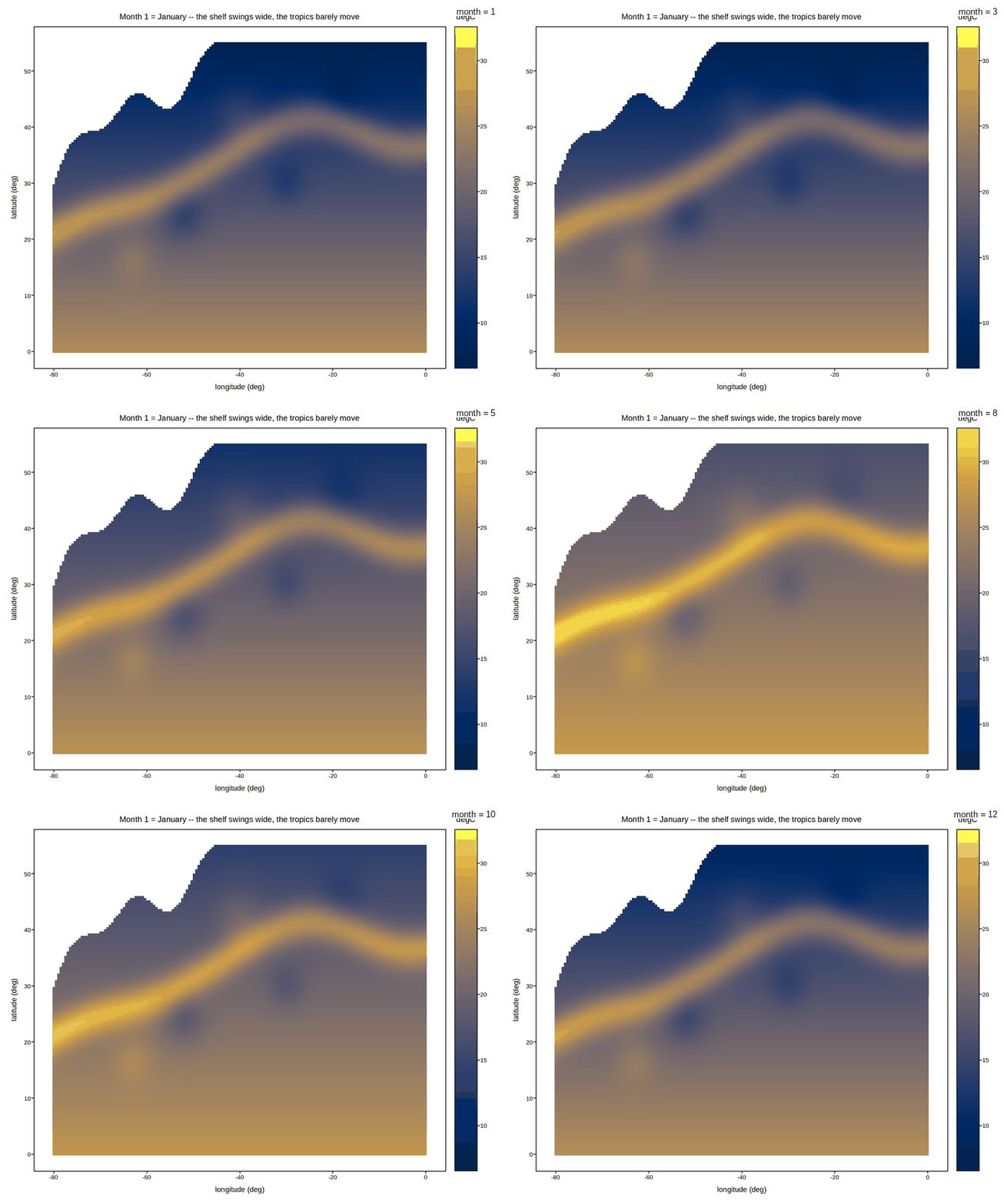
Live figure — pick a tool, then zoom, pan, point-pick or annotate. Nothing is active until a tool is selected.

View this figure’s Vega-Lite export ↗ — the raw JSON spec(s), rendered live by a real Vega-Lite engine.

import os
import tempfile

import numpy as np
import plotpress

lon = np.linspace(-80.0, 0.0, 160)
lat = np.linspace(0.0, 55.0, 140)
LON, LAT = np.meshgrid(lon, lat)

sst_base = 27.0 - 0.28 * LAT
axis = 30.0 + 9.0 * np.tanh((LON + 55.0) / 12.0) + 2.5 * np.sin((LON + 80.0) / 7.0)
sst_base += 9.0 * np.exp(-((LAT - axis) ** 2) / 12.0)
for clon, clat, amp, rad in [(-52.0, 24.0, -3.5, 3.2),
                             (-40.0, 42.0, 3.0, 3.6),
                             (-30.0, 30.0, -2.6, 2.8),
                             (-63.0, 17.0, 2.4, 3.0),
                             (-18.0, 46.0, -2.0, 3.4)]:
    sst_base += amp * np.exp(-((LON - clon) ** 2 + (LAT - clat) ** 2) / (2.0 * rad ** 2))

coast = (30.0 + 0.75 * (LON + 80.0) + 4.0 * np.sin((LON + 80.0) / 6.0)
         + 2.0 * np.sin((LON + 80.0) / 2.3))
land = LAT > coast

# Seasonal amplitude grows with latitude -- the tropics barely move through
# the year, the northern shelf swings widely -- and August runs warmest,
# the ocean's thermal-inertia lag behind the June solstice.
amplitude = 1.0 + 4.0 * (LAT / 55.0)
month = np.arange(1, 13)
sst = np.stack([sst_base + amplitude * np.cos(2.0 * np.pi * (m - 8) / 12.0)
               for m in month])
sst[:, land] = np.nan

fig, ax = plotpress.subplots(figsize=(7.5, 6.0))
mesh = ax.pcolormesh_frames(lon, lat, sst, slider_values=month,
                            slider_label="month", cmap="cividis")
bar = fig.colorbar(mesh, ax=ax)
bar.set_title("degC")
ax.set_xlabel("longitude (deg)")
ax.set_ylabel("latitude (deg)")
ax.set_title("Month 1 = January -- the shelf swings wide, the tropics barely move")
fig.tight_layout()

gif_path = os.path.join(tempfile.gettempdir(), "plotpress_sst_seasonal.gif")
fig.save(gif_path, fps=4)