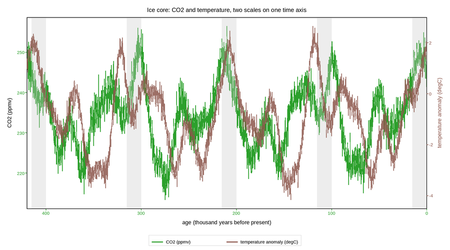
Ice-core CO2 and temperature over four glacial cycles

Two proxies from the same ice core against age: carbon dioxide trapped in air bubbles, and temperature reconstructed from deuterium in the ice itself. They share an x axis and nothing else – different units, different ranges, no common zero – which is exactly what twinx is for.

Twin axes carry a real risk: with two independent y scales, the vertical offset between the curves is an artefact of the limits chosen, and it is easy to manufacture agreement or disagreement by nudging them. The defence used here is to say so, to colour each axis label and its curve to match so no reader has to guess which trace belongs to which scale, and to set both ranges from the data rather than tuning them until the curves overlap prettily.

The x axis runs in thousands of years before present, so it is inverted with invert_xaxis – time then flows left to right the way a reader expects, while the numbers still count backwards the way the field quotes them. The glacial terminations are shaded to give the eye something to align against.

Live figure — pick a tool, then zoom, pan, point-pick or annotate. Nothing is active until a tool is selected.

View this figure’s Vega export ↗ — the raw JSON spec, rendered live by a real Vega engine.

View this figure’s Vega-Lite export ↗ — the raw JSON spec(s), rendered live by a real Vega-Lite engine.

import numpy as np
import polars as pl
import plotpress

rng = np.random.default_rng(11)

age = np.linspace(0.0, 420.0, 3000)               # thousands of years before present

# Glacial cycles: a ~100 kyr sawtooth -- slow descent into glaciation, abrupt
# termination -- rather than a sine, which is the whole point of the record.
phase = (age / 100.0) % 1.0
saw = np.where(phase < 0.85, -phase / 0.85, (phase - 1.0) / 0.15)
saw += 0.25 * np.sin(2 * np.pi * age / 41.0)      # obliquity
saw += 0.12 * np.sin(2 * np.pi * age / 23.0)      # precession

temp = 4.0 * saw + 1.0 + rng.normal(0.0, 0.25, age.size)
# CO2 tracks temperature closely but lags it slightly at terminations.
co2 = 235.0 + 24.0 * np.interp(age, age, saw, left=saw[0]) + 10.0 * saw
co2 = 245.0 + 22.0 * saw + rng.normal(0.0, 2.5, age.size)

CO2_COLOR = "#2ca02c"
TEMP_COLOR = "#8c564b"

# One row per ice-core depth sample -- the shape the two proxy records are
# actually measured and archived in, before either is drawn on its own axis.
core = pl.DataFrame({"age_kyr": age, "co2_ppmv": co2, "temp_anomaly_c": temp})

fig, ax = plotpress.subplots(figsize=(9.0, 5.0))
ax.plot(core["age_kyr"].to_numpy(), core["co2_ppmv"].to_numpy(),
        color=CO2_COLOR, linewidth=1.1, label="CO2 (ppmv)")
ax.set_ylabel("CO2 (ppmv)")
ax.tick_params(labelcolor=CO2_COLOR, color=CO2_COLOR)

ax2 = ax.twinx()
ax2.plot(core["age_kyr"].to_numpy(), core["temp_anomaly_c"].to_numpy(),
         color=TEMP_COLOR, linewidth=1.1, alpha=0.85,
         label="temperature anomaly (degC)")
ax2.set_ylabel("temperature anomaly (degC)")
ax2.tick_params(labelcolor=TEMP_COLOR, color=TEMP_COLOR)

# Terminations: where the sawtooth snaps back upward.
for start in (0.0, 100.0, 200.0, 300.0, 400.0):
    ax.axvspan(start, start + 15.0, color="#cccccc", alpha=0.35)

ax.set_xlim(0.0, 420.0)
ax.invert_xaxis()
ax.set_xlabel("age (thousand years before present)")
ax.set_title("Ice core: CO2 and temperature, two scales on one time axis")
fig.legend(ax=[ax, ax2], loc="lower center", ncol=2)
fig.tight_layout()