Earthquake magnitude-frequency distribution

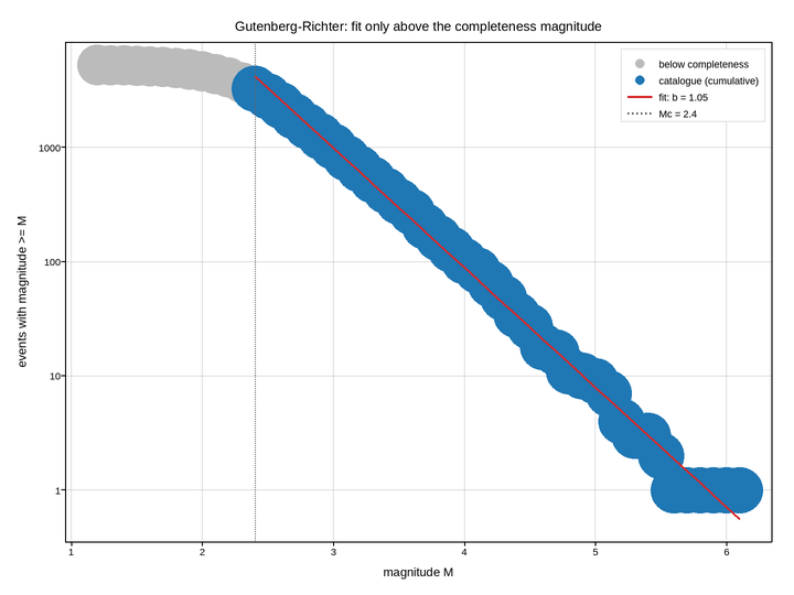
The Gutenberg-Richter law: the number of earthquakes at or above magnitude M in a catalogue falls off as log10 N = a - b M. Plotting it is how seismologists read two numbers straight off a catalogue – the b-value from the slope, and the magnitude of completeness from where the data stops obeying the law.

Everything about the figure follows from that. The counts are cumulative (events at or above each magnitude), because that is the quantity the law describes. The y axis is logarithmic, because a power law is only a straight line there and the eye is far better at judging straightness than curvature. The catalogue spans four decades of event count, so a linear axis would render every magnitude above 5 as indistinguishable from zero.

The roll-off at the small-magnitude end is not physics: it is the network failing to detect small events. Fitting through it would bias b low, so the fit is restricted to M >= Mc and the excluded points are drawn hollow, in a lighter colour, with the cut marked. Showing the discarded data rather than trimming the axis is the honest version – the reader can see the roll-off and judge whether Mc was chosen sensibly.

Live figure — pick a tool, then zoom, pan, point-pick or annotate. Nothing is active until a tool is selected.

View this figure’s Vega export ↗ — the raw JSON spec, rendered live by a real Vega engine.

View this figure’s Vega-Lite export ↗ — the raw JSON spec(s), rendered live by a real Vega-Lite engine.

import numpy as np
import polars as pl
import plotpress

rng = np.random.default_rng(2024)

B_TRUE = 0.98                                     # slope of the law
M_MIN = 1.2                                       # smallest event simulated
M_COMPLETE = 2.4                                  # network detection threshold

# Draw magnitudes from the exponential distribution the law implies, then throw
# away small events with a probability that grows as detection degrades.
n_events = 60000
mags = M_MIN + rng.exponential(1.0 / (B_TRUE * np.log(10.0)), n_events)
detected = rng.random(n_events) < 1.0 / (1.0 + np.exp(-(mags - M_COMPLETE) / 0.18))
mags = mags[detected]

# One row per detected earthquake -- exactly the catalogue a seismic network
# actually publishes, before it is ever binned into a magnitude-frequency
# curve.
catalogue = pl.DataFrame({"magnitude": mags})

bins = np.arange(M_MIN, catalogue["magnitude"].max() + 0.1, 0.1)
mags_arr = catalogue["magnitude"].to_numpy()
cumulative = np.array([(mags_arr >= m).sum() for m in bins], dtype=float)

# One row per magnitude bin of the cumulative curve.
curve = pl.DataFrame({
    "magnitude": bins, "cumulative": cumulative,
}).filter(pl.col("cumulative") > 0).with_columns(
    (pl.col("magnitude") >= M_COMPLETE).alias("complete")
)

complete_curve = curve.filter(pl.col("complete"))
below_curve = curve.filter(~pl.col("complete"))
fit = np.polyfit(complete_curve["magnitude"].to_numpy(),
                 np.log10(complete_curve["cumulative"].to_numpy()), 1)
b_value = -fit[0]

fig, ax = plotpress.subplots(figsize=(7.2, 5.4))
ax.scatter(below_curve["magnitude"].to_numpy(), below_curve["cumulative"].to_numpy(),
           s=26, color="#bbbbbb", label="below completeness")
ax.scatter(complete_curve["magnitude"].to_numpy(), complete_curve["cumulative"].to_numpy(),
           s=30, color="#1f77b4", label="catalogue (cumulative)")
ax.plot(complete_curve["magnitude"].to_numpy(),
        10.0 ** np.polyval(fit, complete_curve["magnitude"].to_numpy()),
        color="#d62728", linewidth=1.6,
        label=f"fit: b = {b_value:.2f}")
ax.axvline(M_COMPLETE, color="#666666", linestyle=":", linewidth=1.2,
           label=f"Mc = {M_COMPLETE:.1f}")

ax.set_yscale("log")
ax.set_xlabel("magnitude M")
ax.set_ylabel("events with magnitude >= M")
ax.set_title("Gutenberg-Richter: fit only above the completeness magnitude")
ax.legend(loc="upper right")
ax.grid(True)
fig.tight_layout()