Zonal-mean atmospheric temperature

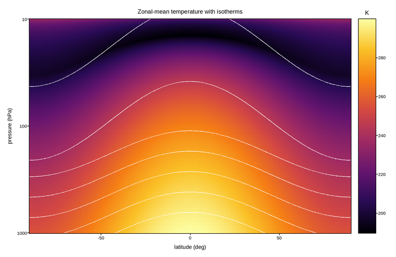
The zonal-mean temperature of the atmosphere against latitude and pressure – the first figure in every dynamics textbook, and the field every reanalysis product is checked against.

Two features fix the structure: temperature falls with height through the troposphere at roughly 6.5 K/km, and the tropopause sits high and cold over the equator (near 100 hPa, below 195 K) but low and warm over the poles. Above it the stratosphere warms again as ozone absorbs sunlight.

Pressure is the vertical coordinate and decreases upward, so the axis is inverted and log-scaled – equal vertical distances then correspond to equal scale heights, which is how the atmosphere actually stacks. Isotherms drawn over the mesh let the tropopause be traced by eye.

Live figure — pick a tool, then zoom, pan, point-pick or annotate. Nothing is active until a tool is selected.

View this figure’s Vega export ↗ — the raw JSON spec, rendered live by a real Vega engine.

View this figure’s Vega-Lite export ↗ — the raw JSON spec(s), rendered live by a real Vega-Lite engine.

/home/runner/work/plotpress/plotpress/docs/applications/earth/plot_05_zonal_mean_temperature.py:54: UserWarning: pcolormesh(): 50 cells along y (e.g. cell 0, y=9.91..10.09) narrower than one output pixel and will not appear in the raster. This mesh has 88400 cells, past the ~2000-cell auto threshold, so rasterized=False will draw every cell exactly but produce a much larger SVG (see pcolormesh_vector_cell_limit.py) -- or use a log scale if this axis spans decades.
  mesh = ax.pcolormesh(lat_axis, pressure_axis, temperature, cmap="inferno")

import numpy as np
import polars as pl
import plotpress

lat = np.linspace(-90.0, 90.0, 340)          # degrees
pressure = np.logspace(np.log10(1000.0), np.log10(10.0), 260)   # hPa
LAT, P = np.meshgrid(lat, pressure)

# Log-pressure height, roughly 7 km per e-fold.
z = 7.0 * np.log(1000.0 / P)

# Surface temperature: warm equator, cold poles.
t_surface = 300.0 - 45.0 * np.sin(np.radians(np.abs(LAT))) ** 2

# Tropopause height: ~17 km at the equator, ~9 km at the poles.
z_trop = 17.0 - 8.0 * np.sin(np.radians(np.abs(LAT))) ** 2

LAPSE = 6.5                                   # K/km through the troposphere
temperature = np.where(
    z < z_trop,
    t_surface - LAPSE * z,
    t_surface - LAPSE * z_trop + 1.8 * (z - z_trop),   # stratospheric inversion
)

# One row per (latitude, pressure) grid point -- sorted before the reshape
# below so the pivot back to a grid is correct regardless of row order.
field = pl.DataFrame({
    "lat": LAT.ravel(), "pressure_hpa": P.ravel(), "temperature": temperature.ravel(),
}).sort(["pressure_hpa", "lat"])

lat_axis = field["lat"].unique().sort().to_numpy()
pressure_axis = field["pressure_hpa"].unique().sort().to_numpy()
temperature = field["temperature"].to_numpy().reshape(pressure_axis.size, lat_axis.size)

fig, ax = plotpress.subplots(figsize=(8.0, 5.2))
mesh = ax.pcolormesh(lat_axis, pressure_axis, temperature, cmap="inferno")
ax.contour(lat_axis, pressure_axis, temperature,
           levels=[200.0, 220.0, 240.0, 260.0, 280.0], colors="white")
fig.colorbar(mesh, ax=ax).set_title("K")
ax.set_yscale("log")
ax.invert_yaxis()
ax.set_xlabel("latitude (deg)")
ax.set_ylabel("pressure (hPa)")
ax.set_title("Zonal-mean temperature with isotherms")
fig.tight_layout()