Doppler radar radial velocity

The velocity product from the same scan as a reflectivity PPI: the component of motion along the beam, positive away from the radar and negative toward it. Forecasters read rotation from it – a tight couplet of inbound beside outbound velocity at the same range is the mesocyclone signature that precedes a tornado.

The sign is the entire meaning, and zero – air moving perpendicular to the beam, or not at all – is physically special. So the map is diverging with limits symmetric about zero, and the zero-isodop line where the colours meet is itself a feature meteorologists trace.

There is a second subtlety the plot has to respect. A pulsed radar can only measure velocity unambiguously up to its Nyquist velocity; faster motion folds, wrapping abruptly from strong outbound to strong inbound. Setting the limits exactly at the Nyquist velocity makes a folded region read as the sharp discontinuity it is, rather than being flattened by autoscaling to whatever extreme the fold produced.

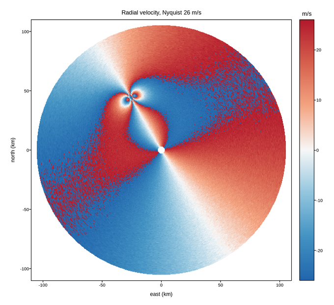
Live figure — pick a tool, then zoom, pan, point-pick or annotate. Nothing is active until a tool is selected.

View this figure’s Vega export ↗ — the raw JSON spec, rendered live by a real Vega engine.

View this figure’s Vega-Lite export ↗ — the raw JSON spec(s), rendered live by a real Vega-Lite engine.

import numpy as np
import polars as pl
import plotpress

rng = np.random.default_rng(61)
NYQUIST = 26.0                                     # m/s

rng_km = np.linspace(3.0, 110.0, 300)
azimuth = np.radians(np.linspace(0.0, 360.0, 361))
R, AZ = np.meshgrid(rng_km, azimuth)
X = R * np.sin(AZ)
Y = R * np.cos(AZ)

# Broad environmental flow from the south-west, sampled along the beam.
beam = np.stack([np.sin(AZ), np.cos(AZ)], axis=-1)
wind = np.array([14.0, 9.0])
radial = beam[..., 0] * wind[0] + beam[..., 1] * wind[1]
radial *= 1.0 + 0.35 * np.log1p(R / 40.0)          # speed increases with height

# A mesocyclone: a small vortex producing an inbound/outbound couplet.
cx, cy, gamma = -26.0, 44.0, 520.0
dx, dy = X - cx, Y - cy
d2 = dx ** 2 + dy ** 2 + 9.0
vx, vy = -gamma * dy / d2, gamma * dx / d2
radial += beam[..., 0] * vx + beam[..., 1] * vy

radial += rng.normal(0.0, 0.8, radial.shape)

# Velocity folding: anything past Nyquist wraps into the opposite sign.
folded = np.angle(np.exp(1j * np.pi * radial / NYQUIST)) * NYQUIST / np.pi
folded[R > 105.0] = np.nan                          # beyond the last gate

# One row per (range, azimuth) radar cell -- sorted before the reshape below
# so the pivot back to a grid is correct regardless of row order. The
# display grid (x, y) is curvilinear, so it is reshaped alongside the
# velocity rather than treated as a separable axis.
scan = pl.DataFrame({
    "range_km": R.ravel(), "azimuth_rad": AZ.ravel(),
    "x": X.ravel(), "y": Y.ravel(), "velocity": folded.ravel(),
}).sort(["azimuth_rad", "range_km"])

grid_shape = (scan["azimuth_rad"].n_unique(), scan["range_km"].n_unique())
X = scan["x"].to_numpy().reshape(grid_shape)
Y = scan["y"].to_numpy().reshape(grid_shape)
folded = scan["velocity"].to_numpy().reshape(grid_shape)

fig, ax = plotpress.subplots(figsize=(6.8, 6.2))
mesh = ax.pcolormesh(X, Y, folded, cmap="RdBu_r", vmin=-NYQUIST, vmax=NYQUIST)
fig.colorbar(mesh, ax=ax).set_title("m/s")
ax.set_aspect("equal")
ax.set_xlabel("east (km)")
ax.set_ylabel("north (km)")
ax.set_title(f"Radial velocity, Nyquist {NYQUIST:.0f} m/s")
fig.tight_layout()