Infrared spectrum with the conventional reversed axes

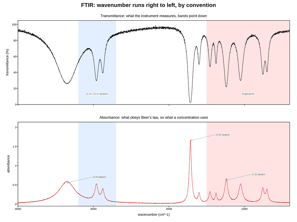
An FTIR transmittance spectrum, drawn with the two inversions the field insists on. Wavenumber decreases left to right, and transmittance is plotted so that absorption bands point downward toward zero. Both look wrong to anyone outside spectroscopy and are immediately readable to anyone inside it, which is the whole argument for honouring a convention rather than improving on it.

Both come from invert_xaxis rather than from negating or reversing the arrays. The distinction matters: the data stays in its natural order, so peak positions can be looked up, sliced and compared without an off-by-one reversal somewhere, and the tick labels still read as wavenumbers rather than as negated ones.

Transmittance is what the instrument measures, but absorbance – its negative logarithm – is what obeys Beer’s law and is proportional to concentration. The second panel shows the same spectrum in absorbance, so a strong band that looks saturated and featureless near 0% transmittance is revealed as the tall, unreliable peak it is. Quoting a concentration from a band that bottoms out here is the classic FTIR error.

The diagnostic regions are shaded and named, because an IR spectrum is read by region before it is read by peak.

Live figure — pick a tool, then zoom, pan, point-pick or annotate. Nothing is active until a tool is selected.

View this figure’s Vega export ↗ — the raw JSON spec, rendered live by a real Vega engine.

View this figure’s Vega-Lite export ↗ — the raw JSON spec(s), rendered live by a real Vega-Lite engine.

import numpy as np
import polars as pl
import plotpress

rng = np.random.default_rng(1800)

wavenumber = np.linspace(400.0, 4000.0, 3600)     # cm^-1

# (centre, peak absorbance, width, name)
BANDS = [
    (3350.0, 0.55, 130.0, "O-H stretch"),
    (2960.0, 0.42, 26.0, None),
    (2875.0, 0.30, 22.0, None),
    (1715.0, 1.65, 18.0, "C=O stretch"),
    (1600.0, 0.24, 16.0, None),
    (1455.0, 0.28, 20.0, None),
    (1375.0, 0.22, 14.0, None),
    (1240.0, 0.62, 26.0, "C-O stretch"),
    (1050.0, 0.48, 30.0, None),
    (755.0, 0.35, 22.0, None),
    (700.0, 0.30, 18.0, None),
]

absorbance = np.zeros_like(wavenumber)
for centre, height, width, _ in BANDS:
    absorbance += height / (1.0 + ((wavenumber - centre) / width) ** 2)
absorbance += 0.02 + 0.015 * np.sin(wavenumber / 400.0)          # sloping baseline
absorbance += rng.normal(0.0, 0.0035, wavenumber.size)

transmittance = 100.0 * 10.0 ** (-np.clip(absorbance, 0.0, None))

# One row per scanned wavenumber -- the shape the FTIR's own interferogram
# export is in, before it is split into transmittance and absorbance panels.
spectrum = pl.DataFrame({
    "wavenumber": wavenumber, "transmittance": transmittance, "absorbance": absorbance,
})
wavenumber = spectrum["wavenumber"].to_numpy()
transmittance = spectrum["transmittance"].to_numpy()
absorbance = spectrum["absorbance"].to_numpy()

REGIONS = [(1500.0, 400.0, "fingerprint", "#ffd7d7"),
           (3200.0, 2700.0, "C-H / O-H stretch", "#d7e8ff")]

fig, axes = plotpress.subplots(2, 1, figsize=(9.6, 7.2), sharex=True)
ax_t, ax_a = axes

for ax in axes:
    for hi, lo, name, color in REGIONS:
        ax.axvspan(lo, hi, color=color, alpha=0.7)

ax_t.plot(wavenumber, transmittance, color="#111111", linewidth=0.9)
ax_t.set_ylabel("transmittance (%)")
ax_t.set_ylim(0.0, 105.0)
ax_t.set_title("Transmittance: what the instrument measures, bands point down")
for hi, lo, name, _ in REGIONS:
    ax_t.text(0.5 * (hi + lo), 12.0, name, ha="center", fontsize=9,
              color="#555555")

ax_a.plot(wavenumber, absorbance, color="#d62728", linewidth=0.9)
ax_a.set_ylim(-0.05, absorbance.max() * 1.28)
ax_a.set_ylabel("absorbance")
ax_a.set_xlabel("wavenumber (cm^-1)")
ax_a.set_title("Absorbance: what obeys Beer's law, so what a concentration uses")
# Offset the labels sideways rather than upward: the tallest band is already at
# the top of the panel, so "above the peak" is off the axes for the one band
# most worth naming.
for centre, height, width, name in BANDS:
    if name:
        ax_a.annotate(name, xy=(centre, height),
                      xytext=(centre - 430.0, height + 0.13),
                      ha="center", fontsize=8, color="#333333",
                      arrowprops={"color": "#888888"})

ax_a.set_xlim(400.0, 4000.0)
ax_a.invert_xaxis()                                # high wavenumber on the left
fig.suptitle("FTIR: wavenumber runs right to left, by convention")
fig.tight_layout()