Electron-ionisation mass spectrum

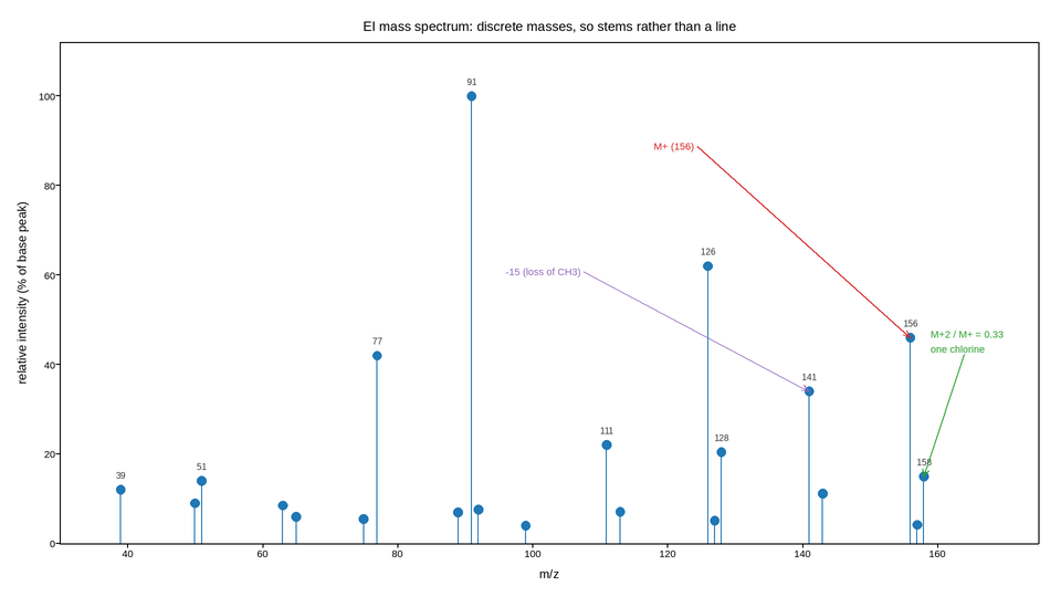
A mass spectrum is a line spectrum: intensity exists at discrete mass-to-charge ratios and is undefined between them. Joining the points with a line would draw signal at m/z values where none was measured, and smooth over the isotope spacing that identifies the elements present. stem is the honest form, and the only one that matches how these spectra are published and searched against libraries.

Intensity is normalised to the base peak at 100%, which is the universal convention – absolute ion counts depend on the source tuning and are not comparable between instruments, so every library entry is relative.

Three features are annotated because they are what an analyst reads first. The molecular ion gives the molecular weight. The M+2 isotope peak at a third of the molecular ion’s height is the signature of one chlorine atom, and its ratio is the measurement, which is why it is labelled with the ratio rather than the height. And the loss of 15 mass units from the molecular ion is a methyl group leaving, which localises where it was attached.

Live figure — pick a tool, then zoom, pan, point-pick or annotate. Nothing is active until a tool is selected.

View this figure’s Vega export ↗ — the raw JSON spec, rendered live by a real Vega engine.

View this figure’s Vega-Lite export ↗ — the raw JSON spec(s), rendered live by a real Vega-Lite engine.

import numpy as np
import polars as pl
import plotpress

# (m/z, relative intensity %) -- fragments of a chlorinated aromatic.
FRAGMENTS = [
    (39, 12.0), (50, 9.0), (51, 14.0), (63, 8.5), (65, 6.0), (75, 5.5),
    (77, 42.0), (89, 7.0), (91, 100.0), (92, 7.6), (99, 4.0),
    (111, 22.0), (113, 7.1), (126, 62.0), (127, 5.1), (128, 20.4),
    (141, 34.0), (143, 11.2), (156, 46.0), (157, 4.2), (158, 15.0),
]
MOLECULAR_ION = 156
BASE_PEAK = 91

# One row per detected fragment ion -- exactly the peak-list table a mass
# spectrometer's own library search exports.
fragments = pl.DataFrame({
    "mz": [m for m, _ in FRAGMENTS],
    "intensity": [i for _, i in FRAGMENTS],
}, schema={"mz": pl.Float64, "intensity": pl.Float64})

fig, ax = plotpress.subplots(figsize=(9.6, 5.4))
ax.stem(fragments["mz"].to_numpy(), fragments["intensity"].to_numpy(),
        linecolor="#1f77b4", markercolor="#1f77b4")

# Label only peaks worth naming: everything above 10% plus the molecular ion.
for row in fragments.iter_rows(named=True):
    m, i = row["mz"], row["intensity"]
    if i >= 12.0 or m == MOLECULAR_ION:
        ax.text(m, i + 2.5, f"{m:.0f}", ha="center", fontsize=8, color="#333333")

m_plus_2 = fragments.filter(pl.col("mz") == MOLECULAR_ION + 2)["intensity"].item()
m_plus_0 = fragments.filter(pl.col("mz") == MOLECULAR_ION)["intensity"].item()

ax.annotate(f"M+ ({MOLECULAR_ION})", xy=(MOLECULAR_ION, m_plus_0),
            xytext=(118.0, 88.0), arrowprops={"color": "#d62728"},
            color="#d62728", fontsize=9)
ax.annotate(f"M+2 / M+ = {m_plus_2 / m_plus_0:.2f}\none chlorine",
            xy=(MOLECULAR_ION + 2, m_plus_2), xytext=(159.0, 46.0),
            arrowprops={"color": "#2ca02c"}, color="#2ca02c", fontsize=9)
ax.annotate("-15 (loss of CH3)", xy=(141.0, 34.0), xytext=(96.0, 60.0),
            arrowprops={"color": "#9467bd"}, color="#9467bd", fontsize=9)

ax.set_xlim(30.0, 175.0)
ax.set_ylim(0.0, 112.0)
ax.set_xlabel("m/z")
ax.set_ylabel("relative intensity (% of base peak)")
ax.set_title("EI mass spectrum: discrete masses, so stems rather than a line")
fig.tight_layout()