Chromatogram with integrated peaks

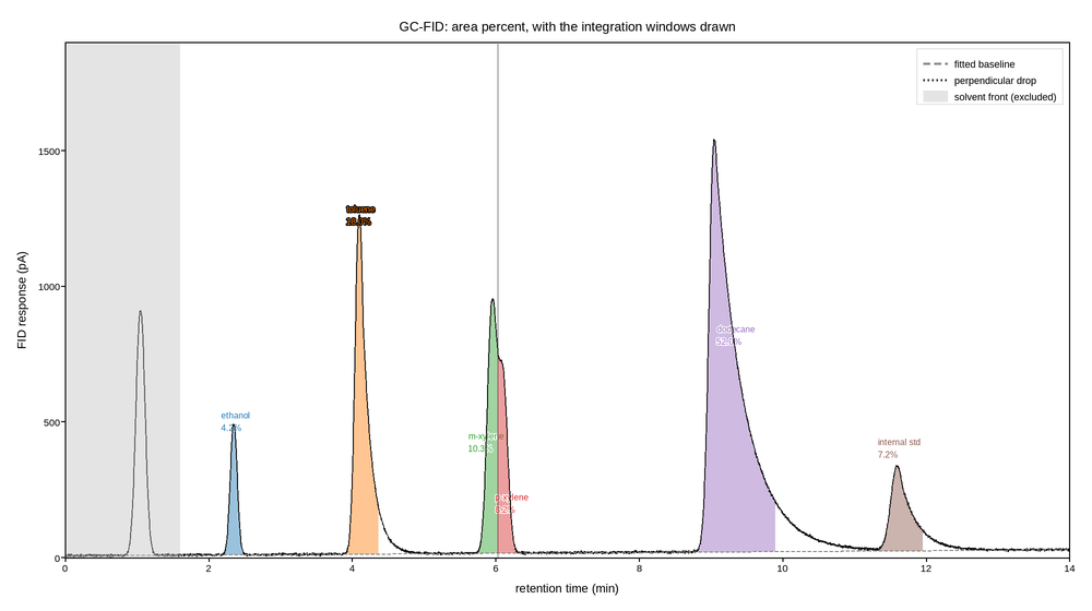
Detector response against retention time from a gas chromatograph, with the integration that turns it into a quantitative result drawn on top. A chromatogram is only data until the peaks are integrated; the areas, not the heights, are proportional to concentration, so the figure has to show which region was assigned to which peak.

That is what the shaded fill_between regions are: each is the area the integrator attributed to one component, bounded below by the fitted baseline. Drawing them makes two common failures visible at a glance. The two coeluting peaks near 6 minutes share a valley rather than returning to baseline, so their split is a perpendicular drop whose position is a judgement call. And the tailing peak at 9 minutes has its own baseline drift, which is why the baseline is a fitted line rather than a constant.

The area percentages are annotated on the peaks rather than tabulated separately, because the number and the peak it came from should not be two lookups apart. The solvent front is excluded from the total – integrating it would swamp everything else – and the figure says so instead of quietly dropping it.

Live figure — pick a tool, then zoom, pan, point-pick or annotate. Nothing is active until a tool is selected.

View this figure’s Vega export ↗ — the raw JSON spec, rendered live by a real Vega engine.

View this figure’s Vega-Lite export ↗ — the raw JSON spec(s), rendered live by a real Vega-Lite engine.

import numpy as np
import polars as pl
import plotpress

rng = np.random.default_rng(9)

t = np.linspace(0.0, 14.0, 4000)                  # minutes

# (retention time, height, width, tailing factor, name)
PEAKS = [
    (2.35, 480.0, 0.045, 1.0, "ethanol"),
    (4.10, 1250.0, 0.055, 1.1, "toluene"),
    # These two are deliberately unresolved: their peaks are closer together
    # than their widths, so the trace never returns to baseline between them.
    (5.95, 890.0, 0.062, 1.0, "m-xylene"),
    (6.10, 640.0, 0.064, 1.0, "p-xylene"),
    (9.05, 1520.0, 0.070, 2.6, "dodecane"),
    (11.60, 310.0, 0.085, 1.3, "internal std"),
]
SOLVENT_FRONT = 1.05


def peak(t, centre, height, width, tail):
    """Exponentially modified Gaussian -- a Gaussian that tails to the right."""
    core = height * np.exp(-((t - centre) ** 2) / (2.0 * width ** 2))
    if tail <= 1.0:
        return core
    decay = np.exp(-np.clip(t - centre, 0.0, None) / (width * tail * 2.2))
    return np.maximum(core, height * decay * np.exp(-np.clip(centre - t, 0, None) ** 2
                                                    / (2 * width ** 2)))


signal = 8.0 + 1.6 * t                             # column bleed: a rising baseline
signal += 900.0 * np.exp(-((t - SOLVENT_FRONT) ** 2) / (2 * 0.06 ** 2))
for centre, height, width, tail, _ in PEAKS:
    signal += peak(t, centre, height, width, tail)
signal += rng.normal(0.0, 2.2, t.size)

baseline = 8.0 + 1.6 * t                           # what the integrator fitted

# One row per detector sample -- the shape the instrument's own trace export
# is in, before any integration window is drawn on it.
trace = pl.DataFrame({"time_min": t, "signal": signal, "baseline": baseline})
t = trace["time_min"].to_numpy()
signal = trace["signal"].to_numpy()
baseline = trace["baseline"].to_numpy()

# Integration windows: back to baseline where possible, a perpendicular drop at
# the valley between the two xylenes.
VALLEY = 6.025
WINDOWS = [(2.15, 2.60), (3.88, 4.36), (5.70, VALLEY), (VALLEY, 6.42),
           (8.80, 9.90), (11.30, 11.95)]
COLORS = ["#1f77b4", "#ff7f0e", "#2ca02c", "#d62728", "#9467bd", "#8c564b"]

areas = []
for lo, hi in WINDOWS:
    sel = (t >= lo) & (t <= hi)
    areas.append(float(np.trapezoid(signal[sel] - baseline[sel], t[sel])))
total = sum(areas)

fig, ax = plotpress.subplots(figsize=(10.0, 5.6))
for (lo, hi), color, area, (_, height, _, _, name) in zip(WINDOWS, COLORS, areas,
                                                          PEAKS):
    sel = (t >= lo) & (t <= hi)
    ax.fill_between(t[sel], baseline[sel], signal[sel], color=color, alpha=0.45)
    centre = 0.5 * (lo + hi)
    ax.text(centre, np.interp(centre, t, signal) + 90.0,
            f"{name}\n{100 * area / total:.1f}%", ha="center", fontsize=8,
            color=color)

ax.plot(t, signal, color="#111111", linewidth=0.9)
ax.plot(t, baseline, color="#888888", linestyle="--", linewidth=1.2,
        label="fitted baseline")
ax.axvline(VALLEY, color="#333333", linestyle=":", linewidth=1.2,
           label="perpendicular drop")
ax.axvspan(0.0, 1.6, color="#bbbbbb", alpha=0.4, label="solvent front (excluded)")

ax.set_xlim(0.0, 14.0)
ax.set_ylim(0.0, 1900.0)
ax.set_xlabel("retention time (min)")
ax.set_ylabel("FID response (pA)")
ax.set_title("GC-FID: area percent, with the integration windows drawn")
ax.legend(loc="upper right")
fig.tight_layout()