Cyclic voltammetry against scan rate

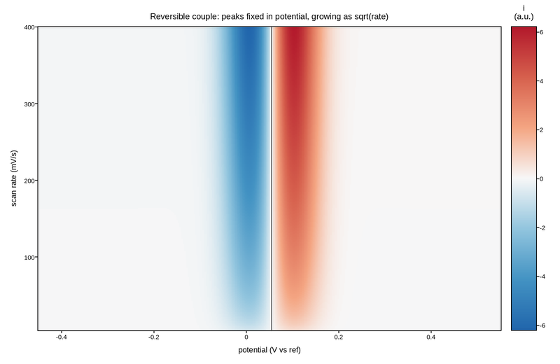
A stack of cyclic voltammograms: measured current against electrode potential and sweep rate. Sweeping the potential back and forth drives a redox couple alternately to oxidation and reduction, and repeating the experiment at different rates is how the kinetics are separated from the thermodynamics.

Faradaic current is signed by definition – anodic current is positive as the species gives up electrons, cathodic negative as it takes them back – and zero current means no reaction is proceeding. That makes a diverging map with symmetric limits the only honest choice; the white band tracks the potentials where the electrode is quiet.

The peak separation stays fixed while peak height grows as the square root of scan rate, the Randles-Sevcik signature of a diffusion-controlled reversible couple. On this map that shows up as the anodic and cathodic ridges staying at constant potential while brightening upward.

Live figure — pick a tool, then zoom, pan, point-pick or annotate. Nothing is active until a tool is selected.

View this figure’s Vega export ↗ — the raw JSON spec, rendered live by a real Vega engine.

View this figure’s Vega-Lite export ↗ — the raw JSON spec(s), rendered live by a real Vega-Lite engine.

import numpy as np
import polars as pl
import plotpress

potential = np.linspace(-0.45, 0.55, 380)      # V vs reference
scan_rate = np.linspace(5.0, 400.0, 300)       # mV/s
E, V = np.meshgrid(potential, scan_rate)

E_HALF = 0.055                                  # formal potential (V)
SEPARATION = 0.059                              # 59 mV for a one-electron couple
WIDTH = 0.045

# Randles-Sevcik: peak current scales with the square root of scan rate.
amplitude = np.sqrt(V / scan_rate.min())

anodic = np.exp(-((E - (E_HALF + SEPARATION / 2)) ** 2) / (2 * WIDTH ** 2))
cathodic = -np.exp(-((E - (E_HALF - SEPARATION / 2)) ** 2) / (2 * WIDTH ** 2))
faradaic = amplitude * (anodic + cathodic)

# Capacitive charging current: proportional to scan rate, and flat in potential.
capacitive = 0.06 * (V / scan_rate.max()) * np.tanh((E - E_HALF) / 0.10)

current = faradaic + capacitive

# One row per swept (potential, scan rate) point -- sorted before the
# reshape below so the pivot back to a grid is correct regardless of order.
sweep = pl.DataFrame({
    "potential_v": E.ravel(),
    "scan_rate_mvs": V.ravel(),
    "current": current.ravel(),
}).sort(["scan_rate_mvs", "potential_v"])

potential_axis = sweep["potential_v"].unique().sort().to_numpy()
scan_rate_axis = sweep["scan_rate_mvs"].unique().sort().to_numpy()
current = sweep["current"].to_numpy().reshape(scan_rate_axis.size, potential_axis.size)
lim = float(sweep["current"].abs().max())

fig, ax = plotpress.subplots(figsize=(8.0, 5.2))
mesh = ax.pcolormesh(potential_axis, scan_rate_axis, current, cmap="RdBu_r",
                     vmin=-lim, vmax=lim)
ax.contour(potential_axis, scan_rate_axis, current, levels=[0.0], colors="#333333")
fig.colorbar(mesh, ax=ax).set_title("i\n(a.u.)")
ax.set_xlabel("potential (V vs ref)")
ax.set_ylabel("scan rate (mV/s)")
ax.set_title("Reversible couple: peaks fixed in potential, growing as sqrt(rate)")
fig.tight_layout()