2-D NMR COSY spectrum

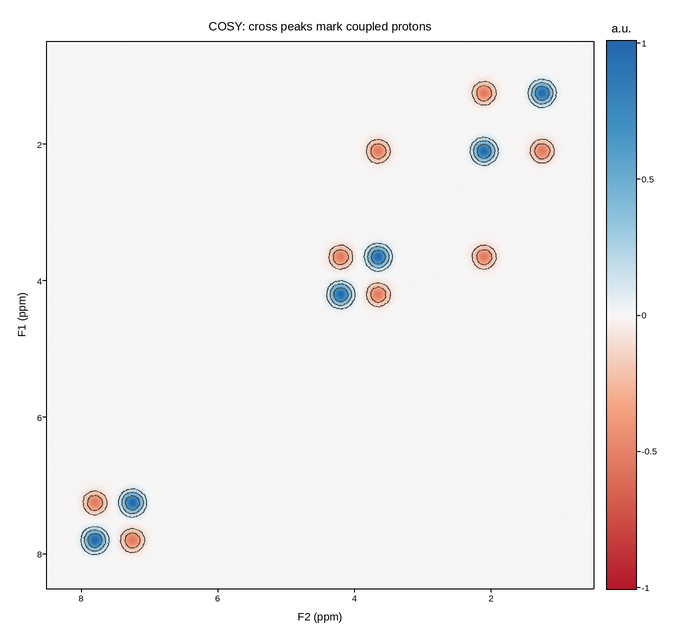
A COSY spectrum: a two-dimensional NMR experiment where cross peaks off the diagonal identify pairs of protons that are scalar-coupled, and so map out which atoms are bonded to which. The diagonal is the ordinary 1-D spectrum; everything interesting is off it.

Phase-sensitive NMR data is signed. Peaks appear with positive and negative lobes, and the sign distinguishes coupling types – so a diverging colour map with limits symmetric about zero is required, not preferred. A sequential map would merge the two lobes of an antiphase multiplet into one blob and discard the information the experiment exists to produce.

Contours over the mesh are how spectroscopists actually read these: peak volumes are integrated from contour levels, and the lowest contour sets what counts as signal above the noise.

Live figure — pick a tool, then zoom, pan, point-pick or annotate. Nothing is active until a tool is selected.

View this figure’s Vega export ↗ — the raw JSON spec, rendered live by a real Vega engine.

View this figure’s Vega-Lite export ↗ — the raw JSON spec(s), rendered live by a real Vega-Lite engine.

import numpy as np
import polars as pl
import plotpress

rng = np.random.default_rng(13)
ppm = np.linspace(0.5, 8.5, 380)          # chemical shift, both dimensions
F1, F2 = np.meshgrid(ppm, ppm)

SHIFTS = [1.25, 2.10, 3.65, 4.20, 7.25, 7.80]
COUPLED = [(0, 1), (2, 3), (4, 5), (1, 2)]     # bonded pairs


def peak(x0, y0, amp, width=0.10):
    """A 2-D Gaussian peak. The width is set so a peak spans several grid
    points -- a real linewidth here would be far narrower than one pixel of
    this map, and would simply not be drawn."""
    return amp * np.exp(-((F1 - x0) ** 2 + (F2 - y0) ** 2) / (2 * width ** 2))


spectrum = np.zeros_like(F1)
for s in SHIFTS:                                # diagonal
    spectrum += peak(s, s, 1.0)
for i, j in COUPLED:                            # symmetric cross peaks
    a, b = SHIFTS[i], SHIFTS[j]
    spectrum += peak(a, b, -0.55) + peak(b, a, -0.55)
spectrum += rng.normal(0.0, 0.006, spectrum.shape)

# One row per (F1, F2) grid point -- sorted before the reshape below so the
# pivot back to a grid is correct regardless of row order.
grid = pl.DataFrame({
    "f1_ppm": F1.ravel(),
    "f2_ppm": F2.ravel(),
    "intensity": spectrum.ravel(),
}).sort(["f2_ppm", "f1_ppm"])

f1_axis = grid["f1_ppm"].unique().sort().to_numpy()
f2_axis = grid["f2_ppm"].unique().sort().to_numpy()
spectrum = grid["intensity"].to_numpy().reshape(f2_axis.size, f1_axis.size)
lim = float(grid["intensity"].abs().max())

fig, ax = plotpress.subplots(figsize=(6.8, 6.4))
mesh = ax.pcolormesh(f1_axis, f2_axis, spectrum, cmap="RdBu", vmin=-lim, vmax=lim)
ax.contour(f1_axis, f2_axis, spectrum, levels=[-0.30, -0.12, 0.12, 0.30, 0.60],
           colors="#444444")
fig.colorbar(mesh, ax=ax).set_title("a.u.")
ax.set_aspect("equal")
ax.invert_xaxis()
ax.invert_yaxis()
ax.set_xlabel("F2 (ppm)")
ax.set_ylabel("F1 (ppm)")
ax.set_title("COSY: cross peaks mark coupled protons")
fig.tight_layout()