Fluorescence excitation-emission matrix

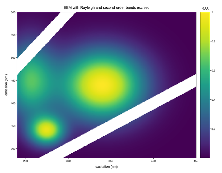
An EEM: fluorescence intensity scanned over both excitation and emission wavelength, used to fingerprint dissolved organic matter in water. Humic-like material fluoresces broadly at long emission wavelengths, protein-like (tryptophan) material in a tighter spot near 280/340 nm.

The measurement has a structural problem that has to be handled before the map means anything. Where emission equals excitation the detector sees Rayleigh scattered excitation light, orders of magnitude above any fluorescence, and at twice the excitation wavelength it sees the second-order grating pass. Those bands carry no fluorescence information and would dominate the colour scale completely.

The standard treatment is to excise them – set them nan – rather than zero them. An unpainted band reads unambiguously as removed data, while a zeroed one looks like a real region of no emission. The colour range is then set by fluorescence alone.

Live figure — pick a tool, then zoom, pan, point-pick or annotate. Nothing is active until a tool is selected.

View this figure’s Vega export ↗ — the raw JSON spec, rendered live by a real Vega engine.

View this figure’s Vega-Lite export ↗ — the raw JSON spec(s), rendered live by a real Vega-Lite engine.

import numpy as np
import polars as pl
import plotpress

excitation = np.linspace(240.0, 450.0, 320)      # nm
emission = np.linspace(280.0, 600.0, 360)        # nm
EX, EM = np.meshgrid(excitation, emission)


def fluorophore(ex0, em0, wex, wem, amp):
    return amp * np.exp(-((EX - ex0) ** 2) / (2 * wex ** 2)
                        - ((EM - em0) ** 2) / (2 * wem ** 2))


eem = (fluorophore(275.0, 340.0, 14.0, 22.0, 0.85)     # tryptophan-like
       + fluorophore(340.0, 440.0, 34.0, 52.0, 1.00)   # humic-like A
       + fluorophore(255.0, 450.0, 20.0, 58.0, 0.62))  # humic-like C

# Scatter bands: first-order Rayleigh, and the second-order grating pass.
eem[np.abs(EM - EX) < 14.0] = np.nan
eem[np.abs(EM - 2.0 * EX) < 18.0] = np.nan

# One row per scanned (excitation, emission) point -- sorted before the
# reshape below so the pivot back to a grid is correct regardless of order.
scan = pl.DataFrame({
    "excitation_nm": EX.ravel(),
    "emission_nm": EM.ravel(),
    "intensity": eem.ravel(),
}).sort(["emission_nm", "excitation_nm"])

excitation_axis = scan["excitation_nm"].unique().sort().to_numpy()
emission_axis = scan["emission_nm"].unique().sort().to_numpy()
eem = scan["intensity"].to_numpy().reshape(emission_axis.size, excitation_axis.size)

fig, ax = plotpress.subplots(figsize=(7.2, 5.6))
mesh = ax.pcolormesh(excitation_axis, emission_axis, eem, cmap="viridis")
fig.colorbar(mesh, ax=ax).set_title("R.U.")
ax.set_xlabel("excitation (nm)")
ax.set_ylabel("emission (nm)")
ax.set_title("EEM with Rayleigh and second-order bands excised")
fig.tight_layout()