SEIR epidemic with an intervention

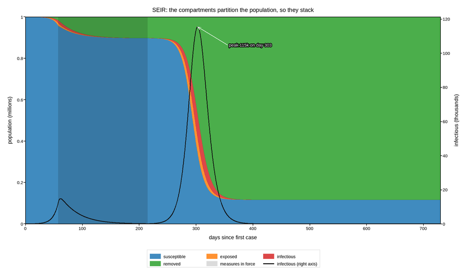
The four compartments of an SEIR model over two years, drawn as a stack. A stack is the right form here for a reason that is easy to state and easy to get wrong: the compartments partition the population, so they sum to a constant, and a stacked area is the only common chart type whose total is itself readable. Four separate lines would show each compartment accurately and hide the fact that they are shares of one fixed whole.

The consequence is that the thickness of each band is its value, not its upper edge – which is why stacks are a poor choice when the reader needs to compare individual series precisely, and a good one when the composition is the point. Infectious cases, the band a reader actually needs to measure, is therefore plotted separately on a twin axis so it can be read against its own scale.

The intervention is drawn where it happens rather than described in the caption. The second wave after the measures are relaxed is the model’s actual output, not a decoration: susceptibles were never depleted enough for the epidemic to end, which is the point the figure is making.

Live figure — pick a tool, then zoom, pan, point-pick or annotate. Nothing is active until a tool is selected.

View this figure’s Vega export ↗ — the raw JSON spec, rendered live by a real Vega engine.

View this figure’s Vega-Lite export ↗ — the raw JSON spec(s), rendered live by a real Vega-Lite engine.

import numpy as np
import polars as pl
import plotpress

POP = 1_000_000
DAYS = 730
dt = 0.25

LATENT = 4.0                                       # days in E
INFECTIOUS = 6.5                                   # days in I
R0_FREE = 2.6
R0_LOCKDOWN = 0.75
INTERVENTION = (58.0, 215.0)                       # days measures are in force

n = int(DAYS / dt) + 1
t = np.linspace(0.0, DAYS, n)
S = np.empty(n); E = np.empty(n); I = np.empty(n); R = np.empty(n)
S[0], E[0], I[0], R[0] = POP - 40.0, 40.0, 0.0, 0.0

for k in range(n - 1):
    inside = INTERVENTION[0] <= t[k] < INTERVENTION[1]
    beta = (R0_LOCKDOWN if inside else R0_FREE) / INFECTIOUS
    new_exposed = beta * S[k] * I[k] / POP
    new_infectious = E[k] / LATENT
    new_removed = I[k] / INFECTIOUS
    S[k + 1] = S[k] + dt * (-new_exposed)
    E[k + 1] = E[k] + dt * (new_exposed - new_infectious)
    I[k + 1] = I[k] + dt * (new_infectious - new_removed)
    R[k + 1] = R[k] + dt * new_removed

# One row per simulated day -- the shape the integrator's own trajectory log
# is in, before any compartment is drawn.
trajectory = pl.DataFrame({
    "day": t, "susceptible": S, "exposed": E, "infectious": I, "removed": R,
})

fig, ax = plotpress.subplots(figsize=(9.6, 5.6))
ax.stackplot(trajectory["day"].to_numpy(),
             trajectory["susceptible"].to_numpy() / 1e6,
             trajectory["exposed"].to_numpy() / 1e6,
             trajectory["infectious"].to_numpy() / 1e6,
             trajectory["removed"].to_numpy() / 1e6,
             colors=["#1f77b4", "#ff7f0e", "#d62728", "#2ca02c"],
             labels=["susceptible", "exposed", "infectious", "removed"],
             alpha=0.85)
ax.axvspan(INTERVENTION[0], INTERVENTION[1], color="#000000", alpha=0.14,
           label="measures in force")

ax2 = ax.twinx()
ax2.plot(trajectory["day"].to_numpy(), trajectory["infectious"].to_numpy() / 1e3,
         color="#111111", linewidth=1.6, label="infectious (right axis)")
ax2.set_ylabel("infectious (thousands)")
ax2.set_ylim(0.0, None)

peak_row = trajectory.sort("infectious", descending=True).row(0, named=True)
# The callout goes where the stack has already settled, not next to the peak:
# beside it is solidly inside the removed band, and black on green is unreadable.
ax2.annotate(f"peak {peak_row['infectious'] / 1e3:.0f}k on day {peak_row['day']:.0f}",
             xy=(peak_row["day"], peak_row["infectious"] / 1e3),
             xytext=(peak_row["day"] + 55.0, peak_row["infectious"] / 1e3 * 0.90),
             arrowprops={"color": "#ffffff"}, fontsize=9,
             color="#ffffff")

ax.set_xlim(0.0, DAYS)
ax.set_ylim(0.0, POP / 1e6)
ax.set_xlabel("days since first case")
ax.set_ylabel("population (millions)")
ax.set_title("SEIR: the compartments partition the population, so they stack")
fig.legend(ax=[ax, ax2], loc="lower center", ncol=3)
fig.tight_layout()