Ramachandran plot as a density map

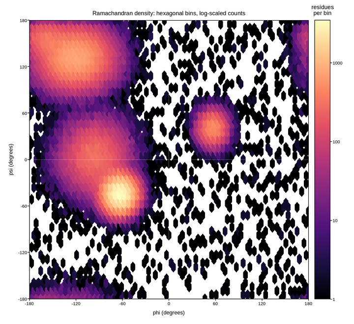
The backbone dihedral angles of every residue in a protein structure database: phi against psi, in degrees. Roughly a quarter of a million points, which settles the plot type on its own – as a scatter it is a black rectangle, and no amount of transparency tuning rescues it, because the interesting features span four orders of magnitude in density.

hexbin bins the points instead of drawing them. Hexagonal bins are used rather than a square grid because a hexagon’s centre is equidistant from all six neighbours, so the bin shape adds no directional bias to a distribution whose features are diagonal ridges – exactly the case where square binning produces visible stair-stepping along the ridge.

The remaining problem is dynamic range: the alpha-helix and beta-sheet basins hold thousands of residues each, the bridge between them holds tens, and the disallowed regions hold the handful that indicate a modelling error. A linear colour scale shows two blobs and nothing else. Colouring the log of the count keeps the basins bright while leaving the sparse allowed regions clearly distinguishable from empty space, which is what a validation reader is looking for.

Live figure — pick a tool, then zoom, pan, point-pick or annotate. Nothing is active until a tool is selected.

View this figure’s Vega export ↗ — the raw JSON spec, rendered live by a real Vega engine.

View this figure’s Vega-Lite export ↗ — the raw JSON spec(s), rendered live by a real Vega-Lite engine.

import numpy as np
import polars as pl
import plotpress

rng = np.random.default_rng(1963)

# Basins: (phi, psi) centre, spread, and share of residues.
BASINS = [
    ((-63.0, -43.0), (11.0, 12.0), 0.42),          # right-handed alpha helix
    ((-120.0, 133.0), (24.0, 20.0), 0.34),         # beta sheet
    ((-95.0, 5.0), (22.0, 24.0), 0.14),            # bridge / polyproline
    ((57.0, 42.0), (10.0, 12.0), 0.055),           # left-handed alpha (rare)
    ((-160.0, 160.0), (14.0, 12.0), 0.04),         # extended corner
]
N = 240_000

phi, psi = [], []
for (cx, cy), (sx, sy), share in BASINS:
    k = int(N * share)
    phi.append(rng.normal(cx, sx, k))
    psi.append(rng.normal(cy, sy, k))
# A thin uniform background: genuine outliers plus a few misbuilt residues.
phi.append(rng.uniform(-180, 180, int(N * 0.005)))
psi.append(rng.uniform(-180, 180, int(N * 0.005)))

phi = np.concatenate(phi)
psi = np.concatenate(psi)
# Dihedrals are circular: wrap back into [-180, 180) rather than clipping.
phi = (phi + 180.0) % 360.0 - 180.0
psi = (psi + 180.0) % 360.0 - 180.0

# One row per residue -- exactly the shape a structure database query
# returns, before the dihedral pairs are ever binned.
residues = pl.DataFrame({"phi": phi, "psi": psi})

fig, ax = plotpress.subplots(figsize=(7.2, 6.6))
# Colour the log of the count: the basins are ~1000x denser than the bridges,
# and on a linear ramp everything but the two basins would be the same colour.
hb = ax.hexbin(residues["phi"].to_numpy(), residues["psi"].to_numpy(),
               gridsize=62, cmap="magma", mincnt=1, norm=plotpress.LogNorm())

bar = fig.colorbar(hb, ax=ax)
bar.set_title("residues\nper bin")

ax.axhline(0.0, color="#ffffff", linewidth=0.6, linestyle=":", alpha=0.6)
ax.axvline(0.0, color="#ffffff", linewidth=0.6, linestyle=":", alpha=0.6)
ax.set_aspect("equal")
ax.set_xlim(-180.0, 180.0)
ax.set_ylim(-180.0, 180.0)
ax.set_xticks([-180, -120, -60, 0, 60, 120, 180])
ax.set_yticks([-180, -120, -60, 0, 60, 120, 180])
ax.set_xlabel("phi (degrees)")
ax.set_ylabel("psi (degrees)")
ax.set_title("Ramachandran density: hexagonal bins, log-scaled counts")
fig.tight_layout()