A pressure pulse bouncing down a rigid duct, animated

An acoustic pulse launched into a closed duct, propagated by direct finite-difference time-domain (FDTD) integration of the 1-D wave equation p_tt = c^2 p_xx rather than an analytic traveling-wave formula – the same leapfrog scheme a room-acoustics or duct-acoustics solver runs, just in one dimension and a few dozen lines. Both ends are rigid (a closed duct, zero particle velocity), enforced with a zero-gradient Neumann boundary that reflects the pulse without inverting it, unlike an open end.

The still gallery image below is the first frame; ax.plot_frames() gives every recorded time step a slider, and fig.save(path, fps=...) exports the whole sequence to a shareable, self-contained GIF – the pulse leaving the source, reflecting off the far wall, passing back through its own path, and reflecting again, is a single continuous replay rather than a series of figures the reader has to mentally stitch together.

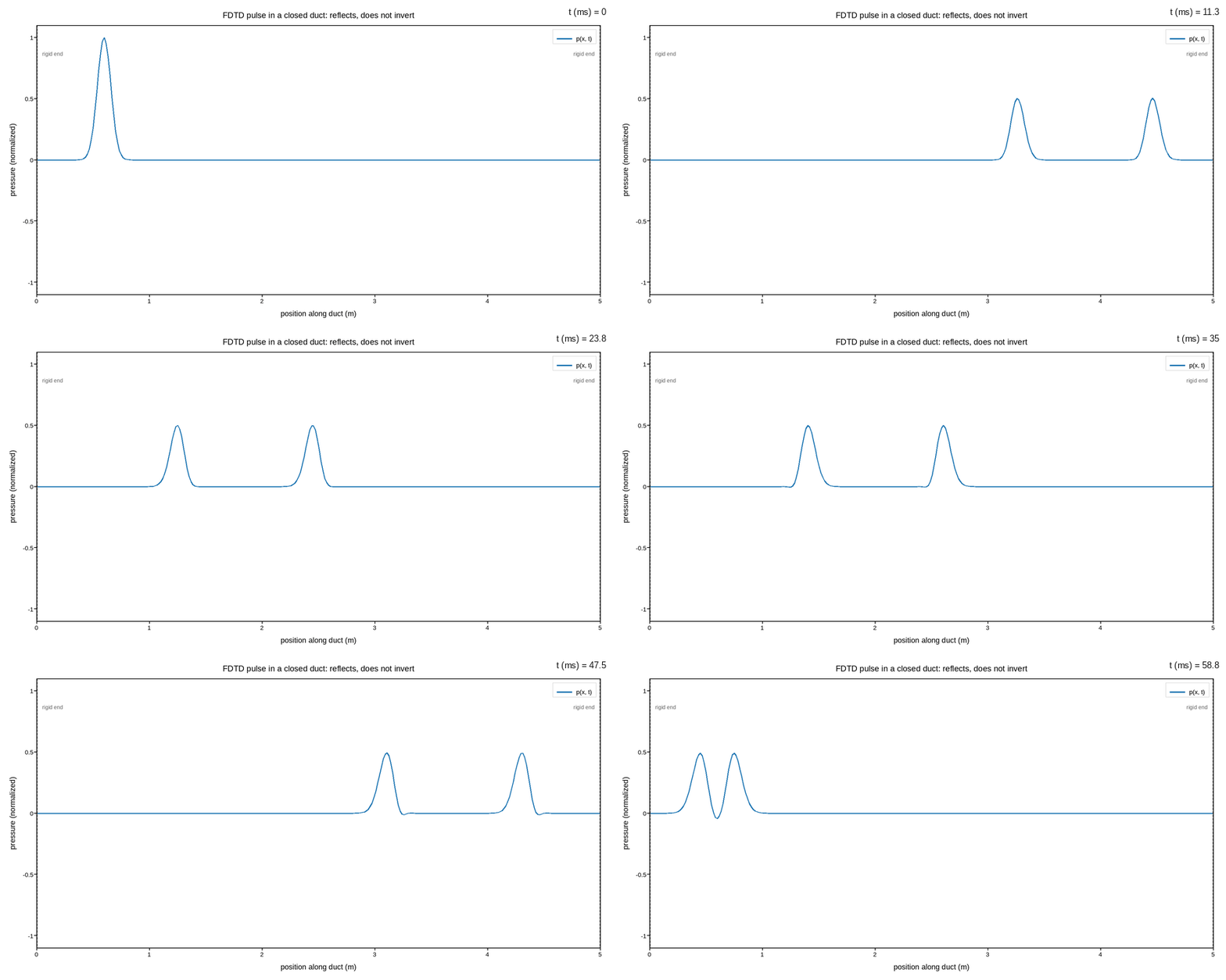
Live figure — pick a tool, then zoom, pan, point-pick or annotate. Nothing is active until a tool is selected.

View this figure’s Vega export ↗ — the raw JSON spec, rendered live by a real Vega engine.

View this figure’s Vega-Lite export ↗ — the raw JSON spec(s), rendered live by a real Vega-Lite engine.

import os
import tempfile

import numpy as np
import plotpress

L = 5.0                                             # duct length (m)
C = 343.0                                           # speed of sound (m/s)
N = 300
x = np.linspace(0.0, L, N)
dx = x[1] - x[0]
CFL = 0.95
dt = CFL * dx / C

# A narrow Gaussian pulse launched near the left end, initially at rest --
# the leapfrog scheme needs two starting levels, and zero initial velocity
# means both are the same profile.
pulse = np.exp(-((x - 0.6) ** 2) / (2 * 0.06 ** 2))
u_prev = pulse.copy()
u_curr = pulse.copy()

N_FRAMES = 48
STEPS_PER_FRAME = 27                                # ~60 ms total: two round trips
frames = np.empty((N_FRAMES, N))
frames[0] = u_curr
r2 = (C * dt / dx) ** 2

for f in range(1, N_FRAMES):
    for _ in range(STEPS_PER_FRAME):
        u_next = np.empty(N)
        u_next[1:-1] = (2 * u_curr[1:-1] - u_prev[1:-1]
                        + r2 * (u_curr[2:] - 2 * u_curr[1:-1] + u_curr[:-2]))
        # Rigid (Neumann) ends: the ghost point mirrors its interior
        # neighbour, so the wall reflects the pulse without inverting it.
        u_next[0] = (2 * u_curr[0] - u_prev[0]
                    + r2 * 2 * (u_curr[1] - u_curr[0]))
        u_next[-1] = (2 * u_curr[-1] - u_prev[-1]
                     + r2 * 2 * (u_curr[-2] - u_curr[-1]))
        u_prev, u_curr = u_curr, u_next
    frames[f] = u_curr

t_ms = np.arange(N_FRAMES) * STEPS_PER_FRAME * dt * 1e3

fig, ax = plotpress.subplots(figsize=(9.0, 4.8))
ax.plot_frames(x, frames, slider_values=t_ms, slider_label="t (ms)",
              color="#1f77b4", label="p(x, t)")
ax.axvline(0.0, color="#333333", linewidth=2.0)
ax.axvline(L, color="#333333", linewidth=2.0)
ax.text(0.05, 0.85, "rigid end", fontsize=8, color="#666666")
ax.text(L - 0.05, 0.85, "rigid end", fontsize=8, color="#666666", ha="right")
ax.set_ylim(-1.1, 1.1)
ax.set_xlim(0.0, L)
ax.set_xlabel("position along duct (m)")
ax.set_ylabel("pressure (normalized)")
ax.set_title("FDTD pulse in a closed duct: reflects, does not invert")
ax.legend(loc="upper right")
fig.tight_layout()

gif_path = os.path.join(tempfile.gettempdir(), "plotpress_duct_pulse.gif")
fig.save(gif_path, fps=20)