Machine vibration spectrum with bearing sidebands

A vibration spectrum from a gearbox, and the reason condition monitoring is done in the frequency domain at all. The overall vibration level of this machine is within limits; the fault is visible only as a pattern of small peaks whose spacing identifies it.

Amplitude spans four decades between the shaft-rate peak and the bearing defect sidebands, so the y axis is logarithmic. This is the case where a log axis is not about convenience: the diagnostic features are 60 dB below the dominant peak, and on a linear axis they are literally sub-pixel.

The x axis is in orders – multiples of shaft speed – rather than hertz. A machine that runs at slightly different speeds between measurements produces peaks at different frequencies but the same orders, so order normalisation is what makes two spectra comparable and what makes “3x shaft rate” a diagnosis rather than an arithmetic exercise.

Families of peaks are marked rather than individual ones. Shaft harmonics, the gear mesh frequency, and the sidebands spaced at the bearing outer-race defect frequency around the mesh are three separate diagnoses, so each gets its own colour of marker. The sidebands are the finding: gear mesh alone is normal, gear mesh flanked by evenly spaced sidebands is a modulated fault.

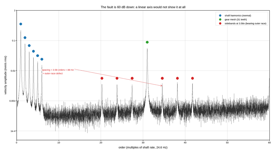
Live figure — pick a tool, then zoom, pan, point-pick or annotate. Nothing is active until a tool is selected.

View this figure’s Vega export ↗ — the raw JSON spec, rendered live by a real Vega engine.

View this figure’s Vega-Lite export ↗ — the raw JSON spec(s), rendered live by a real Vega-Lite engine.

import numpy as np
import polars as pl
import plotpress

rng = np.random.default_rng(3600)

SHAFT_HZ = 24.6
GEAR_TEETH = 31
BPFO = 3.58                                        # bearing defect, in orders

orders = np.linspace(0.2, 60.0, 12000)

# Broadband floor rising slightly with frequency, plus measurement noise.
spectrum = 2.5e-4 * (1.0 + 0.02 * orders) * np.exp(rng.normal(0.0, 0.35,
                                                              orders.size))


def add_peak(order, amplitude, width=0.035):
    global spectrum
    spectrum = spectrum + amplitude / (1.0 + ((orders - order) / width) ** 2)


shaft_orders = np.arange(1, 7)
for k in shaft_orders:
    add_peak(k, 0.22 / k ** 1.5)

add_peak(GEAR_TEETH, 0.055, width=0.05)            # gear mesh
add_peak(2 * GEAR_TEETH - 2, 0.006, width=0.05)

sidebands = [GEAR_TEETH + n * BPFO for n in (-3, -2, -1, 1, 2, 3)]
for order in sidebands:
    add_peak(order, 0.0031, width=0.04)

# One row per frequency-domain bin -- the shape the analyzer's own spectrum
# readout is logged in, before any peak family is picked out of it.
spectrum_table = pl.DataFrame({
    "order": orders,
    "amplitude": spectrum,
})

fig, ax = plotpress.subplots(figsize=(10.4, 5.8))
ax.plot(spectrum_table["order"].to_numpy(), spectrum_table["amplitude"].to_numpy(),
        color="#333333", linewidth=0.7)

ax.scatter(shaft_orders, [0.22 / k ** 1.5 * 1.6 for k in shaft_orders], s=7.0,
           color="#1f77b4", label="shaft harmonics (normal)")
ax.scatter([GEAR_TEETH], [0.055 * 1.6], s=7.0, color="#2ca02c",
           label=f"gear mesh ({GEAR_TEETH} teeth)")
ax.scatter(sidebands, [0.0031 * 1.8] * len(sidebands), s=7.0, color="#d62728",
           label=f"sidebands at {BPFO:.2f}x (bearing outer race)")

ax.annotate(f"spacing = {BPFO:.2f} orders = {BPFO * SHAFT_HZ:.0f} Hz\n"
            "-> outer-race defect",
            xy=(GEAR_TEETH + BPFO, 0.0031), xytext=(6.0, 0.010),
            arrowprops={"color": "#d62728"}, color="#d62728", fontsize=9)

ax.set_yscale("log")
ax.set_xlim(0.0, 60.0)
ax.set_ylim(5e-5, 1.0)
ax.set_xlabel(f"order (multiples of shaft rate, {SHAFT_HZ:.1f} Hz)")
ax.set_ylabel("velocity amplitude (mm/s rms)")
ax.set_title("The fault is 60 dB down: a linear axis would not show it at all")
ax.legend(loc="upper right")
ax.grid(True)
fig.tight_layout()