Reverberation decay and the T60 extrapolation

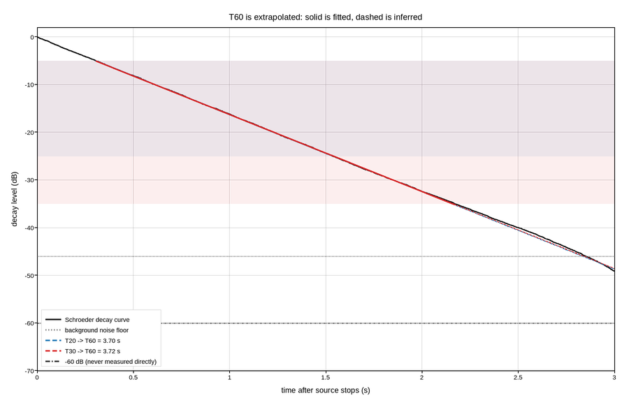
The sound level in a hall after a source is switched off, and the reverberation time extracted from it. The measurement is already logarithmic – decibels – so a linear y axis is the correct one here, and exponential decay appears as a straight line without any transformation.

The number being reported is T60, the time for the level to fall by 60 dB. It is almost never measured directly: the background noise floor is typically only 40 dB below the source, so the last twenty decibels of decay are buried. The standard method fits a straight line over the range that is clean – from 5 dB below the start to 25 or 35 dB below it – and extrapolates. The figure draws the fit range as a shaded band, the fit as a solid line, and the extrapolation beyond the data as a dashed continuation, so the measured part and the inferred part are never confused.

Two evaluation ranges are shown, T20 and T30, both scaled to a 60 dB decay. They agree here, which is the check that the decay really is a single exponential; a hall with a coupled space gives a visibly bent curve and two different answers, and that disagreement is the diagnostic.

The decay is drawn from the backward-integrated impulse response, which is why it is smooth – plotting the raw squared pressure gives a noisy trace whose slope cannot be fitted reliably.

Live figure — pick a tool, then zoom, pan, point-pick or annotate. Nothing is active until a tool is selected.

View this figure’s Vega export ↗ — the raw JSON spec, rendered live by a real Vega engine.

View this figure’s Vega-Lite export ↗ — the raw JSON spec(s), rendered live by a real Vega-Lite engine.

import numpy as np
import polars as pl
import plotpress

rng = np.random.default_rng(1922)

FS = 8000.0
T60_TRUE = 1.85                                    # seconds
NOISE_FLOOR = -46.0                                # dB relative to the start

t = np.arange(0.0, 3.2, 1.0 / FS)

# Impulse response: exponentially decaying noise, plus a stationary noise floor.
decay_rate = 6.9078 / T60_TRUE                     # ln(10^6) / T60
impulse = rng.normal(0.0, 1.0, t.size) * np.exp(-decay_rate * t / 2.0)
impulse += rng.normal(0.0, 10.0 ** (NOISE_FLOOR / 20.0) * 0.55, t.size)

# Schroeder backward integration: integrate the squared response from the end.
energy = np.cumsum(impulse[::-1] ** 2)[::-1]

# One row per time sample of the backward-integrated decay curve -- the
# shape the analyzer actually logs, before any fit range is selected from it.
decay = pl.DataFrame({
    "time_s": t,
    "level_db": 10.0 * np.log10(energy / energy[0]),
})
t = decay["time_s"].to_numpy()
curve = decay["level_db"].to_numpy()

RANGES = [(-5.0, -25.0, "T20", "#1f77b4"), (-5.0, -35.0, "T30", "#d62728")]

fig, ax = plotpress.subplots(figsize=(9.0, 5.8))
ax.plot(t, curve, color="#111111", linewidth=1.3,
        label="Schroeder decay curve")
ax.axhline(NOISE_FLOOR, color="#888888", linestyle=":", linewidth=1.3,
           label="background noise floor")

for k, (top, bottom, name, color) in enumerate(RANGES):
    sel = (curve <= top) & (curve >= bottom)
    coeffs = np.polyfit(t[sel], curve[sel], 1)
    t60 = -60.0 / coeffs[0]

    ax.axhspan(bottom, top, color=color, alpha=0.08)
    ax.plot(t[sel], np.polyval(coeffs, t[sel]), color=color, linewidth=2.2)
    # Beyond the fitted range the line is inference, so it is dashed.
    beyond = np.linspace(t[sel][-1], t60 * 1.02, 60)
    ax.plot(beyond, np.polyval(coeffs, beyond), color=color, linewidth=1.5,
            linestyle="--", label=f"{name} -> T60 = {t60:.2f} s")

ax.axhline(-60.0, color="#333333", linestyle="-.", linewidth=1.2,
           label="-60 dB (never measured directly)")

ax.set_xlim(0.0, 3.0)
ax.set_ylim(-70.0, 2.0)
ax.set_xlabel("time after source stops (s)")
ax.set_ylabel("decay level (dB)")
ax.set_title("T60 is extrapolated: solid is fitted, dashed is inferred")
ax.legend(loc="lower left")
ax.grid(True)
fig.tight_layout()