Sonar range-bearing display

An active sonar ping: echo strength against range and bearing. A hull-mounted array beamforms across bearing and gates the return in time, so the natural grid is polar and the display is drawn on it directly – a curvilinear mesh from 2-D X/Y node arrays.

Two physical effects set the dynamic range. Spreading loss falls as 1/r^2 for a two-way path, and absorption removes a further few dB per kilometre, so raw echo strength from a distant target is orders of magnitude below a nearby one. Sonar therefore applies time-varied gain – amplification that grows with range to compensate the spreading – before display, which is what makes a single colour scale usable across the whole field.

Echo strength after TVG is quoted in dB, so the log is in the data and the colour norm stays linear. Beyond the last gated sample there is no measurement at all, and those cells are nan.

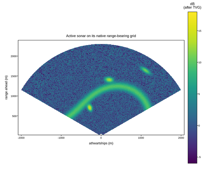
Live figure — pick a tool, then zoom, pan, point-pick or annotate. Nothing is active until a tool is selected.

View this figure’s Vega export ↗ — the raw JSON spec, rendered live by a real Vega engine.

View this figure’s Vega-Lite export ↗ — the raw JSON spec(s), rendered live by a real Vega-Lite engine.

import numpy as np
import polars as pl
import plotpress

rng = np.random.default_rng(53)
rng_m = np.linspace(50.0, 2400.0, 320)                    # slant range (m)
bearing = np.radians(np.linspace(-60.0, 60.0, 300))       # relative bearing
R, B = np.meshgrid(rng_m, bearing)

X = R * np.sin(B)
Y = R * np.cos(B)

# Reverberation background, then discrete targets and a seabed ridge.
echo = rng.rayleigh(1.0, R.shape) * 0.9
for r0, b_deg, strength, spread in [(760.0, -22.0, 26.0, 1.6),
                                    (1420.0, 8.0, 18.0, 1.2),
                                    (1980.0, 34.0, 11.0, 1.0)]:
    b0 = np.radians(b_deg)
    echo += strength * np.exp(-((R - r0) ** 2) / (2 * (28.0 * spread) ** 2)
                              - ((B - b0) ** 2) / (2 * np.radians(2.2) ** 2))
ridge = 1150.0 + 260.0 * np.sin(2.1 * B)
echo += 8.0 * np.exp(-((R - ridge) ** 2) / (2 * 55.0 ** 2))

# Two-way spreading and absorption, then the time-varied gain that undoes them.
spreading = (rng_m[None, :] / rng_m[0]) ** -2.0
absorption = 10.0 ** (-0.06 * (rng_m[None, :] - rng_m[0]) / 1000.0)
received = echo * spreading * absorption
tvg = 1.0 / (spreading * absorption)
db = 10.0 * np.log10(np.maximum(received * tvg, 1e-3))

db[R > 2300.0] = np.nan                    # beyond the last range gate

# One row per ping cell, in its native (range, bearing) coordinates -- sorted
# before the reshape below so the pivot back to a grid is correct regardless
# of row order. The display grid itself (x, y) is curvilinear, so it is
# reshaped alongside db rather than treated as a separable axis.
ping = pl.DataFrame({
    "range_m": R.ravel(),
    "bearing_rad": B.ravel(),
    "x": X.ravel(),
    "y": Y.ravel(),
    "db": db.ravel(),
}).sort(["bearing_rad", "range_m"])

grid_shape = (ping["bearing_rad"].n_unique(), ping["range_m"].n_unique())
X = ping["x"].to_numpy().reshape(grid_shape)
Y = ping["y"].to_numpy().reshape(grid_shape)
db = ping["db"].to_numpy().reshape(grid_shape)

fig, ax = plotpress.subplots(figsize=(7.0, 6.0))
mesh = ax.pcolormesh(X, Y, db, cmap="viridis", vmin=-6.0, vmax=18.0)
fig.colorbar(mesh, ax=ax).set_title("dB\n(after TVG)")
ax.set_aspect("equal")
ax.set_xlabel("athwartships (m)")
ax.set_ylabel("range ahead (m)")
ax.set_title("Active sonar on its native range-bearing grid")
fig.tight_layout()