Josephson parametric amplifier: gain versus pump power and bandwidth

A degenerate parametric amplifier built from a flux-pumped Josephson junction, pumped at twice the signal frequency. Linearizing the equations of motion around the pump gives a closed-form power gain for the amplified quadrature,

G(delta, lambda) = [(1 + lambda)^2 + delta^2] / [(1 - lambda)^2 + delta^2],

where delta is the signal detuning in units of the cavity’s half-linewidth and lambda is the pump strength normalized to the bifurcation threshold. This is the gain-bandwidth trade-off every parametric amplifier lives with, made explicit rather than read off a single spectrum: pushing lambda toward 1 buys gain at line center at the cost of the bandwidth it is usable over, because the denominator only vanishes at delta = 0 in that same limit – the amplifier is heading for its own instability.

The unity-gain contour and the bifurcation line at lambda = 1 are drawn directly on the map, since between them is the entire operating envelope this kind of amplifier is designed within.

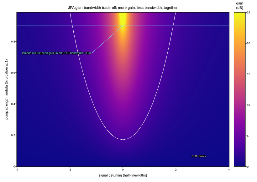
Live figure — pick a tool, then zoom, pan, point-pick or annotate. Nothing is active until a tool is selected.

View this figure’s Vega export ↗ — the raw JSON spec, rendered live by a real Vega engine.

View this figure’s Vega-Lite export ↗ — the raw JSON spec(s), rendered live by a real Vega-Lite engine.

import numpy as np
import polars as pl
import plotpress

detuning = np.linspace(-4.0, 4.0, 380)              # delta, in half-linewidths
pump = np.linspace(0.0, 0.985, 340)                 # lambda, normalized pump strength
DELTA, LAM = np.meshgrid(detuning, pump)

gain = ((1.0 + LAM) ** 2 + DELTA ** 2) / ((1.0 - LAM) ** 2 + DELTA ** 2)
gain_db = 10.0 * np.log10(gain)

# One row per (detuning, pump strength) point -- the shape a swept gain
# characterization is actually logged in, before it is gridded for the mesh.
sweep = pl.DataFrame({
    "detuning": DELTA.ravel(), "lambda_pump": LAM.ravel(), "gain_db": gain_db.ravel(),
}).sort(["lambda_pump", "detuning"])
detuning_axis = sweep["detuning"].unique().sort().to_numpy()
pump_axis = sweep["lambda_pump"].unique().sort().to_numpy()
gain_db_grid = sweep["gain_db"].to_numpy().reshape(pump_axis.size, detuning_axis.size)

fig, ax = plotpress.subplots(figsize=(8.2, 5.8))
mesh = ax.pcolormesh(detuning_axis, pump_axis, gain_db_grid, cmap="plasma",
                     vmin=0.0, vmax=25.0)
bar = fig.colorbar(mesh, ax=ax)
bar.set_title("gain\n(dB)")

ax.contour(detuning_axis, pump_axis, gain_db_grid, levels=[3.0], colors="#ffffff")
ax.text(2.6, 0.06, "3 dB contour", color="#ffffff", fontsize=8)

# 3 dB bandwidth at a representative operating point, read directly off the
# computed row rather than re-derived by hand, so the number on the figure
# is the number the map actually shows.
lam_op = 0.90
row = int(np.argmin(np.abs(pump_axis - lam_op)))
row_db = gain_db_grid[row]
peak_db = row_db.max()
positive = detuning_axis >= 0.0
half_bw = float(np.interp(peak_db - 3.0, row_db[positive][::-1], detuning_axis[positive][::-1]))
ax.axhline(pump_axis[row], color="#7fd8ff", linestyle=":", linewidth=1.1)
ax.annotate(f"lambda = {pump_axis[row]:.2f}: peak gain {peak_db:.0f} dB, "
            f"3 dB bandwidth ~{2 * half_bw:.2f}",
            xy=(0.0, pump_axis[row]), xytext=(-3.8, 0.72),
            arrowprops={"color": "#7fd8ff"}, color="#7fd8ff", fontsize=9)

ax.set_xlabel("signal detuning (half-linewidths)")
ax.set_ylabel("pump strength lambda (bifurcation at 1)")
ax.set_title("JPA gain-bandwidth trade-off: more gain, less bandwidth, together")
fig.tight_layout()