Qubit Rabi chevron

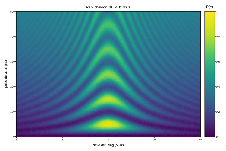
Excited-state population of a driven two-level system, swept over drive detuning and pulse duration – the “chevron” every superconducting-qubit lab measures to calibrate a pi pulse.

On resonance the qubit undergoes full Rabi oscillations at the drive amplitude Omega; off resonance the oscillation is faster but never reaches unity,

P_e = Omega^2 / Omega_eff^2 * sin^2(Omega_eff t / 2), Omega_eff = sqrt(Omega^2 + Delta^2),

which draws the arrowhead fringes. Decoherence damps the contrast toward 1/2 as the pulse lengthens.

A sequential colormap is right here: the data is a probability on a fixed 0..1 scale with no meaningful midpoint, so the limits are pinned to vmin=0, vmax=1 rather than left to autoscale on whatever the sweep happened to reach.

Live figure — pick a tool, then zoom, pan, point-pick or annotate. Nothing is active until a tool is selected.

View this figure’s Vega export ↗ — the raw JSON spec, rendered live by a real Vega engine.

View this figure’s Vega-Lite export ↗ — the raw JSON spec(s), rendered live by a real Vega-Lite engine.

import numpy as np
import polars as pl
import plotpress

RABI_MHZ = 10.0          # drive amplitude on resonance
T2_US = 0.35             # coherence time
rng = np.random.default_rng(3)

detuning = np.linspace(-40.0, 40.0, 320)      # MHz
duration = np.linspace(0.0, 0.5, 260)         # microseconds
D, T = np.meshgrid(detuning, duration)

omega = 2.0 * np.pi * RABI_MHZ                # rad / us
delta = 2.0 * np.pi * D
omega_eff = np.hypot(omega, delta)

contrast = np.exp(-T / T2_US)
p_excited = 0.5 + contrast * (
    (omega ** 2 / omega_eff ** 2) * np.sin(omega_eff * T / 2.0) ** 2 - 0.5)
p_excited += rng.normal(0.0, 0.012, p_excited.shape)   # readout noise

# One row per swept (detuning, duration) shot -- sorted before the reshape
# below so the pivot back to a grid is correct regardless of row order.
sweep = pl.DataFrame({
    "detuning_mhz": D.ravel(),
    "duration_ns": (T * 1e3).ravel(),
    "p_excited": p_excited.ravel(),
}).sort(["duration_ns", "detuning_mhz"])

detuning_axis = sweep["detuning_mhz"].unique().sort().to_numpy()
duration_axis = sweep["duration_ns"].unique().sort().to_numpy()
p_excited = sweep["p_excited"].to_numpy().reshape(duration_axis.size, detuning_axis.size)

fig, ax = plotpress.subplots(figsize=(7.5, 5.0))
mesh = ax.pcolormesh(detuning_axis, duration_axis, p_excited,
                     cmap="viridis", vmin=0.0, vmax=1.0)
bar = fig.colorbar(mesh, ax=ax)
bar.set_title("P(e)")
ax.set_xlabel("drive detuning (MHz)")
ax.set_ylabel("pulse duration (ns)")
ax.set_title(f"Rabi chevron, {RABI_MHZ:.0f} MHz drive")
fig.tight_layout()