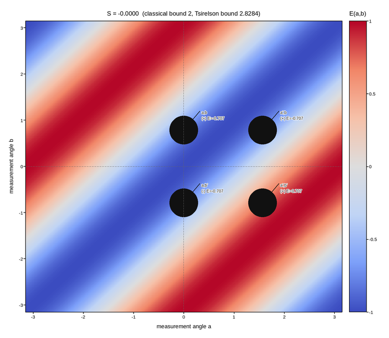
CHSH correlation map: where quantum mechanics beats any local theory

The singlet-state correlation E(a, b) = -cos(a - b) for projective measurements at angles a and b on the two halves of an entangled pair, swept over the full plane of settings. No local hidden-variable theory can reproduce this surface – any theory where each particle carries its own predetermined answer, independent of what the other analyzer is set to, is bounded by the CHSH inequality S <= 2 for

S = E(a, b) - E(a, b’) + E(a’, b) + E(a’, b’),

and the quantum prediction reaches 2 sqrt(2) at the standard optimal settings a=0, a'=pi/2, b=pi/4, b'=-pi/4 – the four points marked on the map. That the four settings sit at regular pi/4 spacings is not a coincidence of this example; it is the geometry that maximizes S for this correlation function, found by extremizing the CHSH combination itself.

Reading S off the four marked points does not require trusting the formula: each E is the map’s own colour at that point, so the number is the map, not an equation quoted beside it.

Live figure — pick a tool, then zoom, pan, point-pick or annotate. Nothing is active until a tool is selected.

View this figure’s Vega export ↗ — the raw JSON spec, rendered live by a real Vega engine.

View this figure’s Vega-Lite export ↗ — the raw JSON spec(s), rendered live by a real Vega-Lite engine.

import numpy as np
import polars as pl
import plotpress

a = np.linspace(-np.pi, np.pi, 340)
b = np.linspace(-np.pi, np.pi, 340)
A, B = np.meshgrid(a, b)
E = -np.cos(A - B)

# One row per (a, b) setting pair -- the shape a Bell-test's own coincidence
# analysis is tabulated in, before it is gridded for the mesh.
table = pl.DataFrame({"a": A.ravel(), "b": B.ravel(), "E": E.ravel()}).sort(["b", "a"])
a_axis = table["a"].unique().sort().to_numpy()
b_axis = table["b"].unique().sort().to_numpy()
E_grid = table["E"].to_numpy().reshape(b_axis.size, a_axis.size)

A0, A1 = 0.0, np.pi / 2.0
B0, B1 = np.pi / 4.0, -np.pi / 4.0


def corr(a_val, b_val):
    return -np.cos(a_val - b_val)


S = corr(A0, B0) - corr(A0, B1) + corr(A1, B0) + corr(A1, B1)

fig, ax = plotpress.subplots(figsize=(7.6, 6.6))
mesh = ax.pcolormesh(a_axis, b_axis, E_grid, cmap="coolwarm", vmin=-1.0, vmax=1.0)
bar = fig.colorbar(mesh, ax=ax)
bar.set_title("E(a,b)")

settings = [("a", A0), ("a'", A1)]
for name_a, va in settings:
    for name_b, vb in [("b", B0), ("b'", B1)]:
        sign = "-" if (name_a, name_b) == ("a", "b'") else "+"
        ax.scatter([va], [vb], s=40.0, color="#111111")
        ax.annotate(f"{name_a},{name_b}\n({sign}) E={corr(va, vb):.3f}",
                    xy=(va, vb), xytext=(va + 0.35, vb + 0.35),
                    fontsize=8, color="#111111", arrowprops={"color": "#111111"})

ax.axhline(0.0, color="#666666", linewidth=0.6)
ax.axvline(0.0, color="#666666", linewidth=0.6)
ax.set_xlabel("measurement angle a")
ax.set_ylabel("measurement angle b")
ax.set_title(f"S = {S:.4f}  (classical bound 2, Tsirelson bound {2 * np.sqrt(2):.4f})")
fig.tight_layout()