Single-qubit RB fidelity across the flux-tuning range

Randomized-benchmarking sequence fidelity, swept over Clifford sequence length and the qubit’s flux bias – connecting gate fidelity directly to the same flux-noise sensitivity that limits coherence away from the sweet spot (Ramsey dephasing across the flux-tuning range). Fidelity still decays exponentially in sequence length at every flux point, so the decay rate alone is what changes: steepest away from the sweet spot, where flux noise dephases each gate a little more, and shallowest at Phi = 0. Plotting the survival probability above its random-circuit asymptote on a log color scale – the same convention Randomized benchmarking of a two-qubit gate uses for its own decay curves – is what keeps the whole family of straight-ish lines legible across two decades at once instead of flattening them all into the same-looking curve near the bottom of a linear scale.

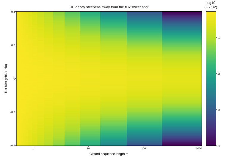
Live figure — pick a tool, then zoom, pan, point-pick or annotate. Nothing is active until a tool is selected.

View this figure’s Vega export ↗ — the raw JSON spec, rendered live by a real Vega engine.

View this figure’s Vega-Lite export ↗ — the raw JSON spec(s), rendered live by a real Vega-Lite engine.

import numpy as np
import polars as pl
import plotpress

ASYMPTOTE = 0.5                    # single qubit: 1/2^n
P0 = 0.9994                          # depolarizing parameter at the sweet spot
FLUX_SENSITIVITY = 0.05              # how much p degrades per (Phi/Phi0)^2
rng = np.random.default_rng(1405)

lengths = np.unique(np.round(np.logspace(0, 3, 26)).astype(int))
flux = np.linspace(-0.4, 0.4, 220)
M, PHI = np.meshgrid(lengths, flux)

p = P0 - FLUX_SENSITIVITY * PHI ** 2
survival = (1.0 - ASYMPTOTE) * p ** M
survival *= 1.0 + rng.normal(0.0, 0.02, survival.shape)
survival = np.clip(survival, 1e-4, 1.0)

# One row per swept (sequence length, flux) point -- sorted before the
# reshape below so the pivot back to a grid is correct regardless of order.
sweep = pl.DataFrame({
    "sequence_length": M.ravel(),
    "flux_phi0": PHI.ravel(),
    "log_survival": np.log10(survival).ravel(),
}).sort(["flux_phi0", "sequence_length"])

lengths_axis = sweep["sequence_length"].unique().sort().to_numpy()
flux_axis = sweep["flux_phi0"].unique().sort().to_numpy()
log_survival = sweep["log_survival"].to_numpy().reshape(flux_axis.size, lengths_axis.size)

fig, ax = plotpress.subplots(figsize=(7.6, 5.4))
mesh = ax.pcolormesh(lengths_axis, flux_axis, log_survival, cmap="viridis")
ax.set_xscale("log")
bar = fig.colorbar(mesh, ax=ax)
bar.set_title("log10\n(F - 1/2)")
ax.set_xlabel("Clifford sequence length m")
ax.set_ylabel("flux bias (Phi / Phi0)")
ax.set_title("RB decay steepens away from the flux sweet spot")
fig.tight_layout()