Wind turbine wake deficit

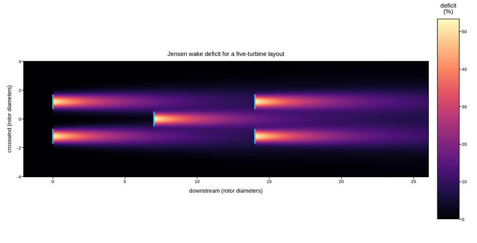
The velocity deficit behind a row of wind turbines: how much slower the air is than the free stream, as a fraction of it. Wake losses decide turbine spacing in a wind farm, so this is the field a layout is optimised against.

Deficit is a positive quantity bounded by construction – a turbine can only slow the flow, never speed it up, and the deficit falls monotonically to zero far downstream. There is no meaningful midpoint, so the map is sequential with the bar anchored at zero. A diverging map would imply a reference deficit that does not exist and would tint undisturbed air as though something had happened to it.

The wakes here follow the Jensen model: a linearly expanding cone whose deficit dilutes with the square of its width. Where two wakes overlap the deficits add in quadrature, which is why the downstream machines sit in noticeably slower air than the front row.

Live figure — pick a tool, then zoom, pan, point-pick or annotate. Nothing is active until a tool is selected.

View this figure’s Vega export ↗ — the raw JSON spec, rendered live by a real Vega engine.

View this figure’s Vega-Lite export ↗ — the raw JSON spec(s), rendered live by a real Vega-Lite engine.

import numpy as np
import polars as pl
import plotpress

D = 120.0                          # rotor diameter (m)
CT = 0.78                          # thrust coefficient
K_WAKE = 0.055                     # wake expansion rate, onshore

x = np.linspace(-2.0 * D, 26.0 * D, 380)      # downstream (m)
y = np.linspace(-4.0 * D, 4.0 * D, 300)       # crosswind (m)
X, Y = np.meshgrid(x, y)

TURBINES = [(0.0, 1.2 * D), (0.0, -1.2 * D),
            (7.0 * D, 0.0), (14.0 * D, 1.2 * D), (14.0 * D, -1.2 * D)]

squared = np.zeros_like(X)
for tx, ty in TURBINES:
    downstream = X - tx
    radius = 0.5 * D + K_WAKE * np.clip(downstream, 0.0, None)
    # Jensen deficit, tapered smoothly across the wake edge.
    core = (1.0 - np.sqrt(1.0 - CT)) * (0.5 * D / radius) ** 2
    inside = np.exp(-((Y - ty) ** 2) / (2 * (radius * 0.62) ** 2))
    deficit = np.where(downstream > 0.0, core * inside, 0.0)
    squared += deficit ** 2                   # quadratic wake superposition

deficit = np.sqrt(squared)

# One row per grid node -- the shape a wake model's own field export is in,
# before it is gridded for the mesh.
field = pl.DataFrame({"x": X.ravel(), "y": Y.ravel(), "deficit": deficit.ravel()}) \
    .sort(["y", "x"])
x = field["x"].unique().sort().to_numpy()
y = field["y"].unique().sort().to_numpy()
deficit = field["deficit"].to_numpy().reshape(y.size, x.size)

fig, ax = plotpress.subplots(figsize=(9.4, 4.8))
mesh = ax.pcolormesh(x / D, y / D, 100.0 * deficit, cmap="magma", vmin=0.0)
fig.colorbar(mesh, ax=ax).set_title("deficit\n(%)")
for tx, ty in TURBINES:                       # rotor discs, to scale
    ax.plot([tx / D, tx / D], [(ty - 0.5 * D) / D, (ty + 0.5 * D) / D],
            color="#00d0ff", linewidth=2.5)
ax.set_aspect("equal")
ax.set_xlabel("downstream (rotor diameters)")
ax.set_ylabel("crosswind (rotor diameters)")
ax.set_title("Jensen wake deficit for a five-turbine layout")
fig.tight_layout()