Generation mix over a week, and net load

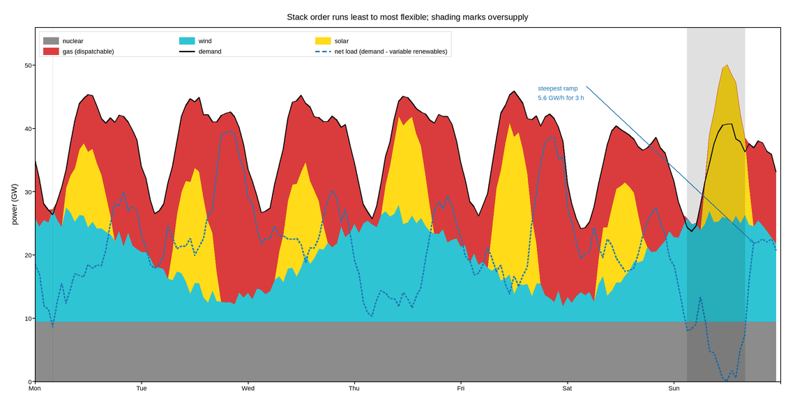
A week of grid generation by source, stacked, with the residual load a dispatchable fleet has to follow drawn over it. The stack order is not arbitrary: sources are laid down from least to most flexible, so the top of the stack is the part that moves to balance the system, which is the part an operator is actually managing.

A stack is the right form because the bands sum to demand, and the reader needs the total and the composition at once. It is the wrong form for comparing two individual sources against each other – the eye judges a band’s thickness poorly when its baseline moves – so the one series that must be read precisely, the net load, is drawn as a line on its own.

The net load is the famous shape: solar output pushes the middle of each day down, and the evening ramp as the sun sets while demand peaks is the steepest thing the fleet is asked to follow. The steepest three-hour ramp of the week is annotated in gigawatts per hour, because that number, not the daily total, is what determines whether the system needs storage.

Negative prices are shaded on the days where generation from must-run sources exceeds demand, which is what the top of the stack crossing the demand line means physically.

Live figure — pick a tool, then zoom, pan, point-pick or annotate. Nothing is active until a tool is selected.

View this figure’s Vega export ↗ — the raw JSON spec, rendered live by a real Vega engine.

View this figure’s Vega-Lite export ↗ — the raw JSON spec(s), rendered live by a real Vega-Lite engine.

import numpy as np
import polars as pl
import plotpress

rng = np.random.default_rng(2023)

HOURS = 24 * 7
t = np.arange(HOURS) / 24.0                        # days

hour_of_day = np.arange(HOURS) % 24
demand = 38.0 + 7.5 * np.sin(2 * np.pi * (hour_of_day - 9.0) / 24.0) \
    + 4.0 * np.sin(4 * np.pi * (hour_of_day - 7.0) / 24.0)
demand *= np.where((np.arange(HOURS) // 24) % 7 < 5, 1.0, 0.90)
demand += rng.normal(0.0, 0.5, HOURS)

# Least flexible first: nuclear is flat, renewables take what they can get,
# gas and hydro follow whatever is left.
nuclear = np.full(HOURS, 9.5)
solar = 26.0 * np.clip(np.sin(np.pi * (hour_of_day - 6.0) / 12.0), 0.0, None)
solar *= np.repeat(rng.uniform(0.45, 1.0, 7), 24)  # cloud cover, day by day
wind = 10.0 + 6.5 * np.sin(2 * np.pi * t / 3.1 + 1.0) + rng.normal(0.0, 0.8, HOURS)
wind = np.clip(wind, 0.5, None)

must_run = nuclear + solar + wind
gas = np.clip(demand - must_run, 0.0, None)
curtailed = np.clip(must_run - demand, 0.0, None)

net_load = demand - solar - wind                   # what the dispatchable fleet sees

# One row per hour of the week -- the shape a grid operator's own dispatch
# log is in, before it is stacked or the steepest ramp is picked out of it.
dispatch = pl.DataFrame({
    "day": t, "demand": demand, "nuclear": nuclear, "wind": wind, "solar": solar,
    "gas": gas, "curtailed": curtailed, "net_load": net_load,
})
t = dispatch["day"].to_numpy()
net_load = dispatch["net_load"].to_numpy()
curtailed = dispatch["curtailed"].to_numpy()

fig, ax = plotpress.subplots(figsize=(11.4, 5.8))
ax.stackplot(t, dispatch["nuclear"].to_numpy(), dispatch["wind"].to_numpy(),
             dispatch["solar"].to_numpy(), dispatch["gas"].to_numpy(),
             colors=["#7f7f7f", "#17becf", "#ffd700", "#d62728"],
             labels=["nuclear", "wind", "solar", "gas (dispatchable)"],
             alpha=0.9)
ax.plot(t, dispatch["demand"].to_numpy(), color="#111111", linewidth=1.6,
        label="demand")
ax.plot(t, net_load, color="#1f77b4", linewidth=2.0, linestyle="--",
        label="net load (demand - variable renewables)")

# Steepest three-hour ramp in the week.
ramp = (net_load[3:] - net_load[:-3]) / 3.0
k = int(np.argmax(ramp))
ax.annotate(f"steepest ramp\n{ramp[k]:.1f} GW/h for 3 h",
            xy=(t[k + 3], net_load[k + 3]), xytext=(t[k] - 1.9, 46.0),
            arrowprops={"color": "#1f77b4"}, color="#1f77b4", fontsize=9)

for day in range(7):
    over = curtailed[day * 24:(day + 1) * 24]
    if over.max() > 0.5:
        lo = day + np.argmax(over > 0.5) / 24.0
        hi = day + (23 - np.argmax(over[::-1] > 0.5)) / 24.0
        ax.axvspan(lo, hi, color="#000000", alpha=0.12)

ax.set_xlim(0.0, 7.0)
ax.set_ylim(0.0, 56.0)
ax.set_xticks(np.arange(8), ["Mon", "Tue", "Wed", "Thu", "Fri", "Sat", "Sun", ""])
ax.set_ylabel("power (GW)")
ax.set_title("Stack order runs least to most flexible; shading marks oversupply")
ax.legend(loc="upper left", ncol=3)
fig.tight_layout()