Battery capacity fade and coulombic efficiency

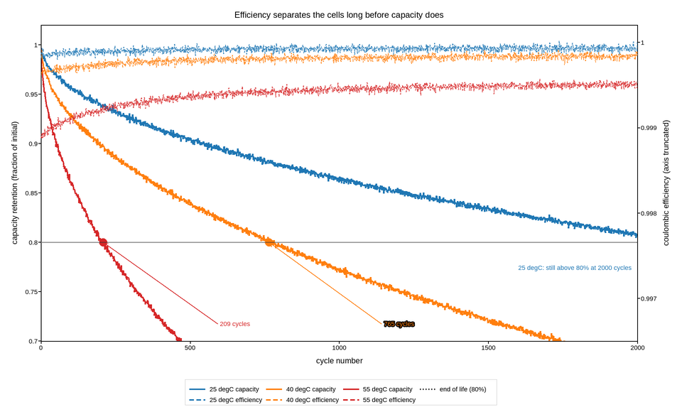
Two thousand cycles of a lithium-ion cell at three temperatures, with the quantity that predicts failure plotted alongside the quantity that measures it.

Capacity fade is on the left axis and is what everyone looks at, but by the time it moves the damage is done. Coulombic efficiency – charge out divided by charge in on each cycle – is on the right axis, and its distance below unity is a direct measure of how much lithium is being consumed by side reactions per cycle. It separates the three temperatures hundreds of cycles before the capacity curves do, which is the argument the figure makes.

The efficiency axis is the interesting design problem. The values live between 0.997 and 1.000, so an axis starting at zero would render all three cells as the same flat line at the top. The axis is therefore deliberately truncated and labelled to say so, because a truncated axis that does not announce itself is how a 0.2% difference gets presented as a dramatic one.

End of life is conventionally 80% of initial capacity, so that threshold is a reference line, and the cycle at which each cell crosses it is annotated. The 40 degC cell has not crossed within the test, so its life is quoted as a bound rather than extrapolated – the fade is visibly not linear, and extrapolating a sublinear curve linearly overstates the life.

Live figure — pick a tool, then zoom, pan, point-pick or annotate. Nothing is active until a tool is selected.

View this figure’s Vega export ↗ — the raw JSON spec, rendered live by a real Vega engine.

View this figure’s Vega-Lite export ↗ — the raw JSON spec(s), rendered live by a real Vega-Lite engine.

import numpy as np
import polars as pl
import plotpress

rng = np.random.default_rng(2018)

cycles = np.arange(1, 2001)
EOL = 0.80

CELLS = [
    # temperature, fade coefficient, efficiency deficit, colour
    (25, 0.0043, 6.0e-5, "#1f77b4"),
    (40, 0.0072, 1.4e-4, "#ff7f0e"),
    (55, 0.0139, 4.2e-4, "#d62728"),
]

fig, ax = plotpress.subplots(figsize=(9.6, 5.8))
ax2 = ax.twinx()

for temp, k, deficit, color in CELLS:
    # Capacity fade goes as the square root of cycle count while SEI growth
    # dominates -- diffusion-limited, so sublinear, not a straight line.
    capacity = 1.0 - k * np.sqrt(cycles)
    capacity += rng.normal(0.0, 0.0016, cycles.size)

    efficiency = 1.0 - deficit * (1.0 + 400.0 / (cycles + 250.0))
    efficiency += rng.normal(0.0, 2.5e-5, cycles.size)

    # One row per charge/discharge cycle -- the shape the cycler's own log
    # is in, before the end-of-life cycle is picked out of it.
    log = pl.DataFrame({"cycle": cycles, "capacity": capacity, "efficiency": efficiency})

    ax.plot(log["cycle"].to_numpy(), log["capacity"].to_numpy(), color=color,
            linewidth=1.8, label=f"{temp} degC capacity")
    ax2.plot(log["cycle"].to_numpy(), log["efficiency"].to_numpy(), color=color,
             linewidth=1.1, linestyle="--", alpha=0.85, label=f"{temp} degC efficiency")

    below = log.filter(pl.col("capacity") <= EOL)
    if below.height:
        n_eol = below["cycle"][0]
        ax.scatter([n_eol], [EOL], s=8.0, color=color)
        # Both callouts sit on the one clear band below every curve. They all
        # point at the same horizontal line, so placing each beside its own
        # crossing put them on top of each other and on the traces.
        ax.annotate(f"{n_eol} cycles", xy=(n_eol, EOL),
                    xytext=(600.0 if n_eol < 600 else 1150.0, 0.715),
                    color=color, fontsize=9, arrowprops={"color": color})
    else:
        ax.text(1980.0, EOL - 0.028,
                f"{temp} degC: still above {EOL:.0%} at {cycles[-1]} cycles",
                fontsize=9, color=color, ha="right")

ax.axhline(EOL, color="#333333", linestyle=":", linewidth=1.4,
           label="end of life (80%)")

ax.set_xlim(0.0, 2000.0)
ax.set_ylim(0.70, 1.02)
ax.set_xlabel("cycle number")
ax.set_ylabel("capacity retention (fraction of initial)")

# Truncated on purpose: the whole signal lives in the last 0.3%.
ax2.set_ylim(0.9965, 1.0002)
ax2.set_ylabel("coulombic efficiency (axis truncated)")

ax.set_title("Efficiency separates the cells long before capacity does")
fig.legend(ax=[ax, ax2], loc="lower center", ncol=4)
fig.tight_layout()