Resistivity pseudosection (LogNorm)

An apparent-resistivity pseudosection from a DC resistivity survey: electrode separation sets the depth of investigation, so plotting against position and pseudo-depth gives a first look at the subsurface before any inversion.

Earth resistivity spans an enormous range – clay and brine at a few ohm-metre, saturated sands in the tens, dry gravel and crystalline bedrock in the thousands. Four orders of magnitude on a linear scale reduces everything below the resistive basement to a single dark tone, which is why resistivity is conventionally plotted, contoured and inverted in the log domain. LogNorm does that in the colour mapping, and the colorbar ticks land on decades.

The data is strictly positive, which is what makes a log scale admissible.

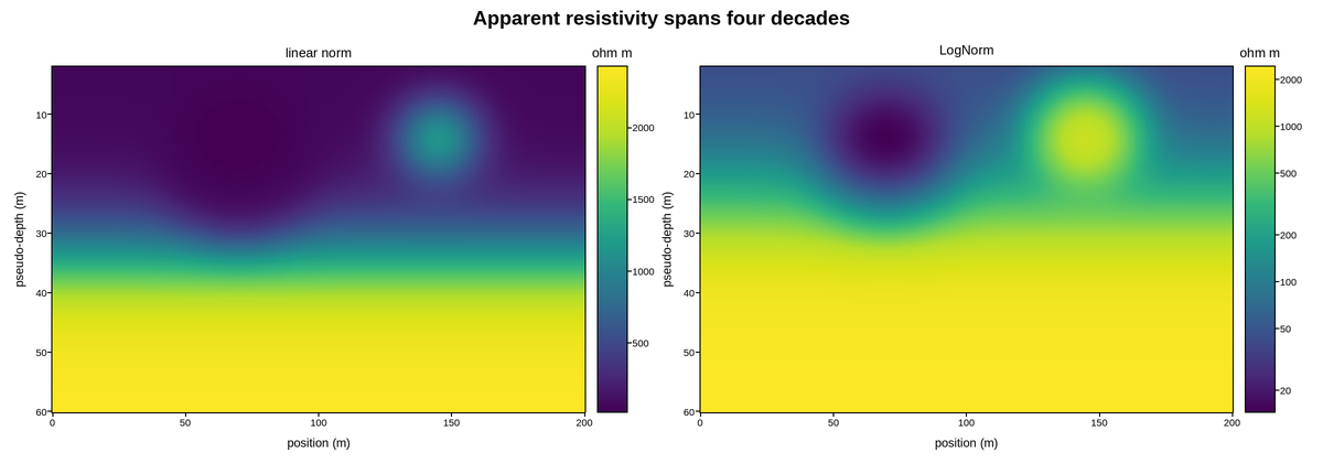
Live figure — pick a tool, then zoom, pan, point-pick or annotate. Nothing is active until a tool is selected.

View this figure’s Vega export ↗ — the raw JSON spec, rendered live by a real Vega engine.

View this figure’s Vega-Lite export ↗ — the raw JSON spec(s), rendered live by a real Vega-Lite engine.

import numpy as np
import polars as pl
import plotpress

x = np.linspace(0.0, 200.0, 340)          # electrode position (m)
depth = np.linspace(2.0, 60.0, 260)       # pseudo-depth (m)
X, D = np.meshgrid(x, depth)

# Layered background: conductive overburden, resistive basement beneath.
rho = 40.0 * np.ones_like(X)
rho *= 1.0 + 60.0 / (1.0 + np.exp(-(D - 34.0) / 5.0))

# A conductive clay lens and a resistive boulder field.
rho /= 1.0 + 6.0 * np.exp(-((X - 70.0) ** 2) / 380.0 - ((D - 18.0) ** 2) / 70.0)
rho *= 1.0 + 14.0 * np.exp(-((X - 145.0) ** 2) / 260.0 - ((D - 12.0) ** 2) / 40.0)

# One row per (position, pseudo-depth) sounding -- sorted before the reshape
# below so the pivot back to a grid is correct regardless of row order.
soundings = pl.DataFrame({
    "position_m": X.ravel(), "depth_m": D.ravel(), "resistivity": rho.ravel(),
}).sort(["depth_m", "position_m"])

x_axis = soundings["position_m"].unique().sort().to_numpy()
depth_axis = soundings["depth_m"].unique().sort().to_numpy()
rho = soundings["resistivity"].to_numpy().reshape(depth_axis.size, x_axis.size)

fig, axes = plotpress.subplots(1, 2, figsize=(12.0, 4.2))
linear = axes[0].pcolormesh(x_axis, depth_axis, rho, cmap="viridis")
axes[0].set_title("linear norm")
fig.colorbar(linear, ax=axes[0]).set_title("ohm m")

log = axes[1].pcolormesh(x_axis, depth_axis, rho, cmap="viridis", norm=plotpress.LogNorm())
axes[1].set_title("LogNorm")
fig.colorbar(log, ax=axes[1]).set_title("ohm m")

for ax in axes:
    ax.invert_yaxis()
    ax.set_xlabel("position (m)")
    ax.set_ylabel("pseudo-depth (m)")
fig.suptitle("Apparent resistivity spans four decades")
fig.tight_layout()