Service latency percentiles over a day

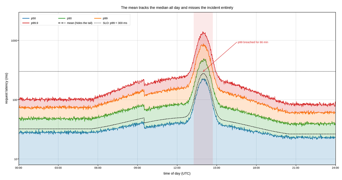
Request latency for a web service through one day, as percentiles rather than as a mean. The mean is drawn too, and its job in this figure is to be visibly useless: it sits near the median all day and says nothing about the incident at 14:00 that a fifth of users experienced.

Latency distributions are heavy-tailed, so a summary that averages over the tail hides it by construction. Percentiles do not: p99 is the experience of the worst 1% of requests, and it is a real user’s experience, not a statistical artefact. Plotting p50, p90, p99 and p99.9 as a fan makes the shape of the tail visible, and the widening of the fan is the thing to react to.

The y axis is logarithmic because the percentiles span two decades. On a linear axis p50 and p90 collapse onto the x axis whenever p99.9 spikes, so the ordinary user experience becomes unreadable exactly when something is going wrong.

The bands between adjacent percentiles are filled rather than left as four lines, which turns the gap between p50 and p99 – the tail spread – into an area the eye can compare across the day. The SLO is a reference line, and the window where p99 breached it is shaded, because the SLO is defined on a percentile and the breach is the event the on-call engineer is paged for.

Live figure — pick a tool, then zoom, pan, point-pick or annotate. Nothing is active until a tool is selected.

View this figure’s Vega export ↗ — the raw JSON spec, rendered live by a real Vega engine.

View this figure’s Vega-Lite export ↗ — the raw JSON spec(s), rendered live by a real Vega-Lite engine.

import numpy as np
import polars as pl
import plotpress

rng = np.random.default_rng(503)

MINUTES = 24 * 60
t = np.arange(MINUTES) / 60.0
SLO_MS = 300.0

# Diurnal load, a deploy at 09:30 that helps, and an incident at 14:00.
load = 0.45 + 0.55 * np.clip(np.sin(np.pi * (t - 5.5) / 15.0), 0.0, None)
base = 26.0 * (1.0 + 0.9 * load ** 3)
base *= np.where(t > 9.5, 0.82, 1.0)               # a deploy that helped
incident = 1.0 + 4.6 * np.exp(-((t - 14.0) ** 2) / (2 * 0.42 ** 2))

# Log-normal service times: the tail multiplier grows when the system saturates.
spread = 0.28 + 0.30 * load
percentiles = [(50, "#1f77b4"), (90, "#2ca02c"), (99, "#ff7f0e"),
               (99.9, "#d62728")]
Z = {50: 0.0, 90: 1.2816, 99: 2.3263, 99.9: 3.0902}

curves = {}
for p, _ in percentiles:
    value = base * incident * np.exp(Z[p] * spread)
    value *= np.exp(rng.normal(0.0, 0.035, MINUTES))
    curves[p] = value

mean = base * incident * np.exp(0.5 * spread ** 2) * 1.05

# One row per minute of the day -- the shape the monitoring system's own
# time series export is in, before it is split into percentile bands.
timeseries = pl.DataFrame({
    "hour": t,
    "p50": curves[50], "p90": curves[90], "p99": curves[99], "p99_9": curves[99.9],
    "mean": mean,
})
t = timeseries["hour"].to_numpy()

fig, ax = plotpress.subplots(figsize=(11.0, 5.8))

previous = np.full(MINUTES, 8.0)
for p, color in percentiles:
    col = f"p{p:g}".replace(".", "_")
    values = timeseries[col].to_numpy()
    ax.fill_between(t, previous, values, color=color, alpha=0.20)
    ax.plot(t, values, color=color, linewidth=1.6, label=f"p{p:g}")
    previous = values

ax.plot(t, timeseries["mean"].to_numpy(), color="#111111", linewidth=1.4,
        linestyle="--", label="mean (hides the tail)")
ax.axhline(SLO_MS, color="#333333", linestyle=":", linewidth=1.6,
           label=f"SLO: p99 < {SLO_MS:.0f} ms")

breach = timeseries["p99"].to_numpy() > SLO_MS
if breach.any():
    lo, hi = t[breach][0], t[breach][-1]
    ax.axvspan(lo, hi, color="#d62728", alpha=0.10)
    ax.annotate(f"p99 breached for {(hi - lo) * 60:.0f} min",
                xy=(0.5 * (lo + hi), SLO_MS), xytext=(16.6, 900.0),
                arrowprops={"color": "#d62728"}, color="#d62728", fontsize=9)

ax.set_yscale("log")
ax.set_xlim(0.0, 24.0)
ax.set_ylim(8.0, 3000.0)
ax.set_xticks(np.arange(0, 25, 3), [f"{h:02d}:00" for h in range(0, 25, 3)])
ax.set_xlabel("time of day (UTC)")
ax.set_ylabel("request latency (ms)")
ax.set_title("The mean tracks the median all day and misses the incident entirely")
ax.legend(loc="upper left", ncol=3)
ax.grid(True)
fig.tight_layout()