UV-vis spectrum through a first-order reaction, animated

A spectrophotometer parked on one sample while A -> B runs to completion, recording a full spectrum every few seconds instead of a single wavelength. Absorbance is additive (Beer-Lambert, one path length shared by both species), so the measured spectrum at any instant is just the concentration-weighted sum of each species’ own spectrum,

A(lambda, t) = eps_A(lambda) [A](t) + eps_B(lambda) [B](t),

with [A](t) decaying and [B](t) rising as simple first-order exponentials. The animation is the point: a static before/after pair shows that the reaction happened, but only watching the whole spectrum morph shows how – one continuous family of curves rather than a jump between two.

Every curve in the family passes through the same point regardless of how far the reaction has run: the isosbestic point, where the two species’ spectra happen to cross and so contribute equally no matter the mixture. A single clean isosbestic point is itself a diagnostic chemists rely on – it is the signature of a clean two-species conversion, and a second reaction step or a stray intermediate is exactly what smears it into a band instead of a point.

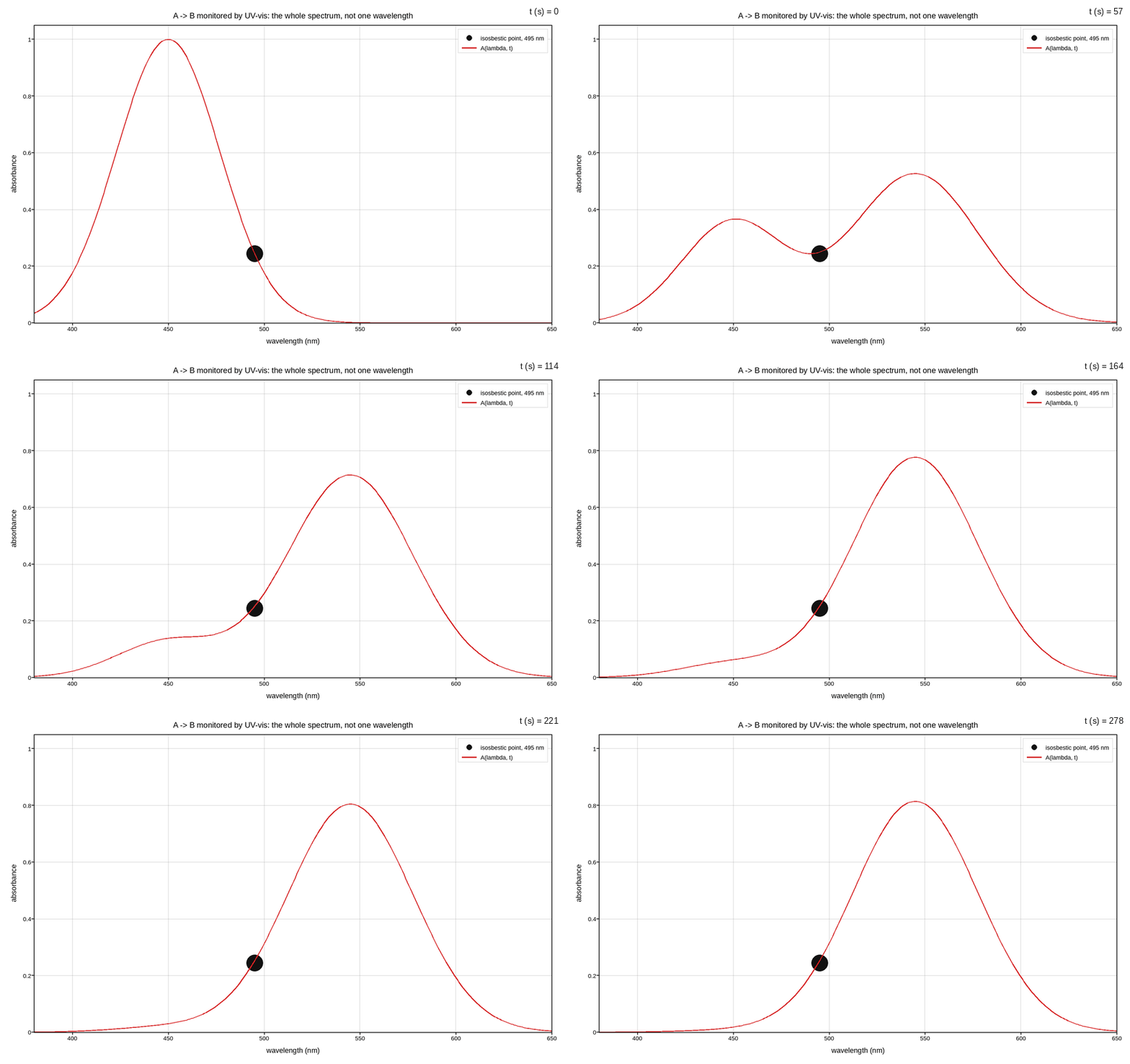
Live figure — pick a tool, then zoom, pan, point-pick or annotate. Nothing is active until a tool is selected.

View this figure’s Vega export ↗ — the raw JSON spec, rendered live by a real Vega engine.

View this figure’s Vega-Lite export ↗ — the raw JSON spec(s), rendered live by a real Vega-Lite engine.

import os
import tempfile

import numpy as np
import plotpress

K = 0.018                                           # first-order rate constant (1/s)
A0 = 1.0                                             # initial concentration

wavelength = np.linspace(380.0, 650.0, 320)          # nm
eps_A = 1.00 * np.exp(-((wavelength - 450.0) / 38.0) ** 2)
eps_B = 0.82 * np.exp(-((wavelength - 545.0) / 46.0) ** 2)

N_FRAMES = 40
t = np.linspace(0.0, 5.0 / K, N_FRAMES)              # out to ~5 half-lives
conc_A = A0 * np.exp(-K * t)
conc_B = A0 * (1.0 - np.exp(-K * t))

# One row per (time, wavelength) sample -- the shape a diode-array
# spectrophotometer's own kinetics run is recorded in, before the frame
# family is pivoted out of it.
absorbance = conc_A[:, None] * eps_A[None, :] + conc_B[:, None] * eps_B[None, :]

# The isosbestic point: where the two pure-species spectra themselves cross,
# independent of the kinetics -- read directly off eps_A/eps_B, not fitted.
# Restricted to between the two peak centres, since both spectra also fade
# to ~0 out at the domain edges, which is not a crossing in any real sense.
between = (wavelength > 450.0) & (wavelength < 545.0)
cross = np.arange(wavelength.size)[between][
    np.argmin(np.abs(eps_A[between] - eps_B[between]))]

fig, ax = plotpress.subplots(figsize=(8.6, 5.4))
ax.scatter([wavelength[cross]], [eps_A[cross]], s=18.0, color="#111111",
          label=f"isosbestic point, {wavelength[cross]:.0f} nm")
ax.plot_frames(wavelength, absorbance, slider_values=t, slider_label="t (s)",
              color="#d62728", label="A(lambda, t)")
ax.set_xlim(380.0, 650.0)
ax.set_ylim(0.0, 1.05)
ax.set_xlabel("wavelength (nm)")
ax.set_ylabel("absorbance")
ax.set_title("A -> B monitored by UV-vis: the whole spectrum, not one wavelength")
ax.legend(loc="upper right")
ax.grid(True)
fig.tight_layout()

gif_path = os.path.join(tempfile.gettempdir(), "plotpress_kinetics_spectrum.gif")
fig.save(gif_path, fps=12)