Electric dipole potential (SymLogNorm)

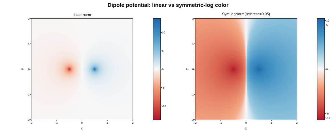
Fields that change sign and span decades defeat a linear color scale. The potential of a +q / -q pair is dominated by the two poles: linearly normalized, everything beyond them washes out to the midpoint and the dipole’s structure disappears.

SymLogNorm is logarithmic in each direction away from zero and linear through a narrow band around it, so the near field and the far field are legible at once. Pair it with a diverging colormap so the sign is visible and zero sits at the neutral midpoint.

Live figure — pick a tool, then zoom, pan, point-pick or annotate. Nothing is active until a tool is selected.

View this figure’s Vega export ↗ — the raw JSON spec, rendered live by a real Vega engine.

View this figure’s Vega-Lite export ↗ — the raw JSON spec(s), rendered live by a real Vega-Lite engine.

import numpy as np
import polars as pl
import plotpress

g = np.linspace(-2.0, 2.0, 320)
X, Y = np.meshgrid(g, g)

HALF_SEP = 0.5           # charges at x = +/- HALF_SEP
SOFTEN = 0.06            # keeps the poles finite on a discrete grid
potential = (1.0 / (np.hypot(X - HALF_SEP, Y) + SOFTEN)
             - 1.0 / (np.hypot(X + HALF_SEP, Y) + SOFTEN))

# One row per field-point sample -- sorted before the reshape below so the
# pivot back to a grid is correct regardless of row order.
field = pl.DataFrame({
    "x": X.ravel(),
    "y": Y.ravel(),
    "potential": potential.ravel(),
}).sort(["y", "x"])

x_axis = field["x"].unique().sort().to_numpy()
y_axis = field["y"].unique().sort().to_numpy()
V = field["potential"].to_numpy().reshape(y_axis.size, x_axis.size)

fig, axes = plotpress.subplots(1, 2, figsize=(11.0, 4.4))
linear = axes[0].pcolormesh(x_axis, y_axis, V, cmap="RdBu")
axes[0].set_title("linear norm")
fig.colorbar(linear, ax=axes[0])

symlog = axes[1].pcolormesh(x_axis, y_axis, V, cmap="RdBu",
                            norm=plotpress.SymLogNorm(linthresh=0.05))
axes[1].set_title("SymLogNorm(linthresh=0.05)")
fig.colorbar(symlog, ax=axes[1])

for ax in axes:
    ax.set_aspect("equal")
    ax.set_xlabel("x")
    ax.set_ylabel("y")
fig.suptitle("Dipole potential: linear vs symmetric-log color")
fig.tight_layout()