Reload a figure’s titles, labels, and axis settings, not just its data

load_data()’s "template" entry carries more than grid shape: every axes’ own title, x/y labels, limits, scale, grid, and legend settings, plus the figure’s own suptitle – see plotpress.figure_from_template()’s docstring for the full list. Replotting recovered data into a rebuilt figure never needs a single set_title()/set_xlabel()/set_xlim() call written by hand; only a legend (which needs labeled data to already exist) is re-applied explicitly, using the exact settings load_data() already captured.

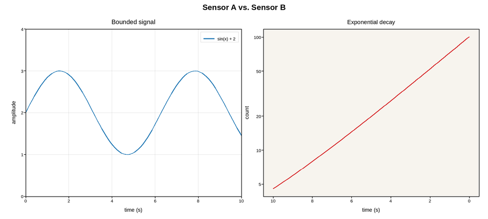
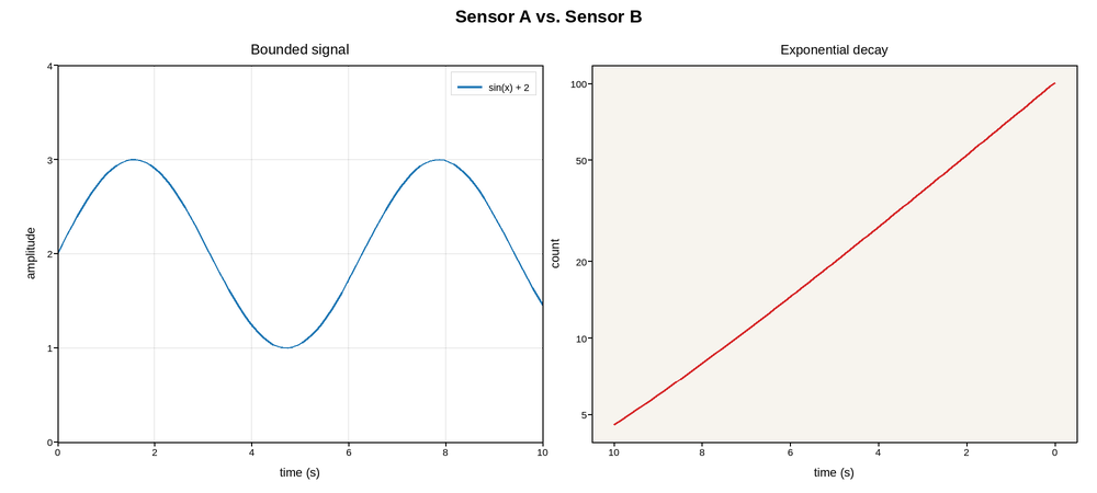
The source figure below is deliberately decorated with everything this covers, to make the point concretely: the two figures this script renders – source_fig (built directly) and rebuilt_fig (loaded back from its own saved HTML, then replotted) – render to byte-identical SVG.

• 
• 

Live figure — pick a tool, then zoom, pan, point-pick or annotate. Nothing is active until a tool is selected.

View this figure’s Vega export ↗ — the raw JSON spec, rendered live by a real Vega engine.

View this figure’s Vega-Lite export ↗ — the raw JSON spec(s), rendered live by a real Vega-Lite engine.

Live figure — pick a tool, then zoom, pan, point-pick or annotate. Nothing is active until a tool is selected.

View this figure’s Vega export ↗ — the raw JSON spec, rendered live by a real Vega engine.

View this figure’s Vega-Lite export ↗ — the raw JSON spec(s), rendered live by a real Vega-Lite engine.

import os
import tempfile

import numpy as np
import plotpress


def _build_source():
    """A two-panel figure using most of what figure_from_template() now
    reproduces: title/fontsize, x/y labels, explicit limits, a log y-scale,
    a styled grid, an inverted x-axis, a per-axes facecolor, a legend, and
    a figure-wide suptitle."""
    fig, (left, right) = plotpress.subplots(1, 2, figsize=(10, 4.5))

    x = np.linspace(0, 10, 100)
    left.plot(x, np.sin(x) + 2, label="sin(x) + 2")
    left.set_title("Bounded signal", fontsize=13)
    left.set_xlabel("time (s)"); left.set_ylabel("amplitude")
    left.set_xlim(0, 10); left.set_ylim(0, 4)
    left.grid(True, alpha=0.3)
    left.legend(loc="upper right", framealpha=0.9)

    y = np.exp(-x / 3) * 100 + 1
    right.plot(x, y, color="C3")
    right.set_title("Exponential decay")
    right.set_xlabel("time (s)"); right.set_ylabel("count")
    right.set_yscale("log")
    right.invert_xaxis()
    right.set_facecolor("#f7f4ee")

    fig.suptitle("Sensor A vs. Sensor B", size=16)
    fig.tight_layout()
    return fig


source_fig = _build_source()
path = os.path.join(tempfile.gettempdir(), "plotpress_gallery_full_decorations.html")
source_fig.save(path, interactive=True)

# ---------------------------------------------------------------------------
# Load it back and rebuild -- no title, label, limit, scale, or grid is
# re-typed anywhere below; figure_from_template() already applied all of it
# to `left2`/`right2` by the time this loop starts. The one exception is
# the legend: it draws from already-plotted, labeled artists, so it has to
# be called again *after* replotting -- with the exact settings
# load_data() already captured, not re-guessed.
# ---------------------------------------------------------------------------
entry = plotpress.load_data(path)["Figure 1"]
template, axes_data = entry["template"], entry["axes"]

rebuilt_fig, (left2, right2) = plotpress.figure_from_template(template)

left_series = axes_data["Bounded signal"]["series"][0]
left2.plot(left_series["x"], left_series["y"], label="sin(x) + 2")
left2.legend(**template["axes"][0]["legend"])

right_series = axes_data["Exponential decay"]["series"][0]
right2.plot(right_series["x"], right_series["y"], color="C3")

rebuilt_fig.tight_layout()

# The point of this example: the two renders match exactly, not just
# visually -- see tests/test_svg_output.py's own
# test_reconstructed_figure_renders_byte_identical_svg_to_the_original for
# the same claim as an enforced regression test.
assert rebuilt_fig.to_svg() == source_fig.to_svg()