Density tails and the cut parameter

cut extends each density past the observed extremes by that many bandwidths. The default cut=0 clips the silhouette at the data range, which is honest about where observations stop; cut=2 lets the tails taper the way seaborn draws them.

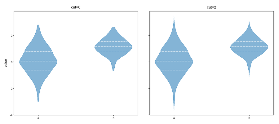
Live figure — pick a tool, then zoom, pan, point-pick or annotate. Nothing is active until a tool is selected.

View this figure’s Vega export ↗ — the raw JSON spec, rendered live by a real Vega engine.

View this figure’s Vega-Lite export ↗ — the raw JSON spec(s), rendered live by a real Vega-Lite engine.

import numpy as np
import plotpress

rng = np.random.default_rng(4)
groups = [rng.normal(loc, s, 300) for loc, s in [(0.0, 1.0), (1.2, 0.6)]]

fig, axes = plotpress.subplots(1, 2, figsize=(9.0, 4.0), sharey=True)
for ax, cut in zip(axes, [0.0, 2.0]):
    ax.violinplot(groups, cut=cut, inner="quartile")
    ax.set_xticks([1, 2])
    ax.set_xticklabels(["a", "b"])
    ax.set_title(f"cut={cut:g}")
axes[0].set_ylabel("value")
fig.tight_layout()