Density over a histogram

The classic distplot combination: a density-normalised histogram with the kernel-density estimate drawn on top, so both share a y axis.

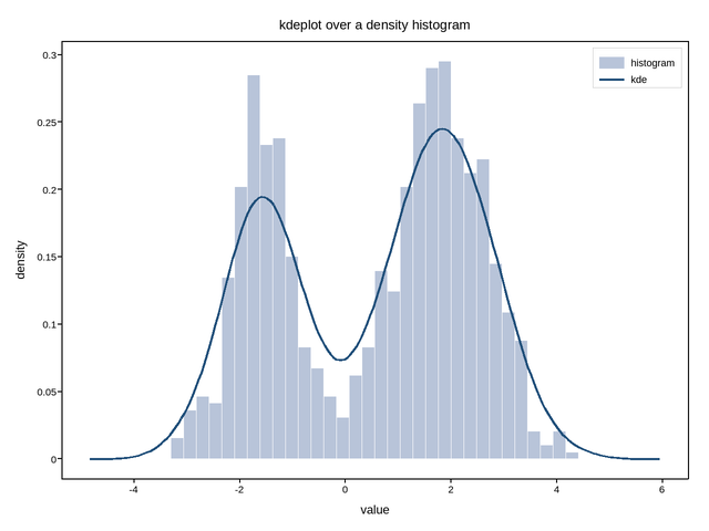
Live figure — pick a tool, then zoom, pan, point-pick or annotate. Nothing is active until a tool is selected.

View this figure’s Vega export ↗ — the raw JSON spec, rendered live by a real Vega engine.

View this figure’s Vega-Lite export ↗ — the raw JSON spec(s), rendered live by a real Vega-Lite engine.

import numpy as np
import plotpress

rng = np.random.default_rng(3)
# Bimodal, where a single smooth curve and the raw bins disagree usefully.
values = np.concatenate([rng.normal(-1.6, 0.6, 300), rng.normal(1.8, 0.9, 500)])

fig, ax = plotpress.subplots()
ax.hist(values, bins=32, density=True, color="#b8c4d9", label="histogram")
ax.kdeplot(values, color="#1f4e79", linewidth=2.0, label="kde")
ax.set_xlabel("value")
ax.set_ylabel("density")
ax.set_title("kdeplot over a density histogram")
ax.legend()
fig.tight_layout()