Density estimates: binned above a few thousand points

kdeplot and violinplot compute an exact kernel sum for small samples, but that sum builds a grid x n intermediate that dominates as the sample grows (~0.9 s and 20M floats at 100k points, and too large to allocate at all near a million). Above a few thousand observations they switch to linear binning: the data is binned onto the grid once and the result convolved with the kernel, so the cost stops scaling with sample size.

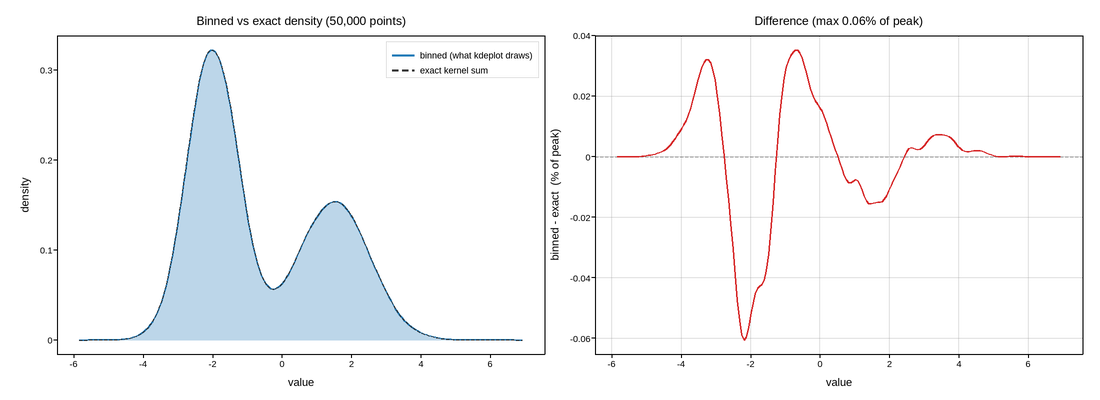
The binned curve is an approximation of the exact one. This example shows how close it is, and where it is least accurate.

import numpy as np
import plotpress

rng = np.random.default_rng(0)

# Bimodal, and large enough (> 4000 points) that kdeplot uses linear binning.
data = np.concatenate([rng.normal(-2.0, 0.7, 30_000),
                       rng.normal(1.5, 1.0, 20_000)])

fig, (ax1, ax2) = plotpress.subplots(1, 2, figsize=(11, 4))

# kdeplot returns the *binned* estimate for a sample this size.
binned = ax1.kdeplot(data, fill=True, label="binned (what kdeplot draws)")

# The exact per-point kernel sum, on the same grid, for comparison. This is the
# textbook estimator kdeplot uses directly below the size threshold. The
# bandwidth is Silverman's rule -- the same value kdeplot computes internally.
grid = binned.x
bw = 1.06 * data.std(ddof=1) * data.size ** (-1 / 5)
u = (grid[:, None] - data[None, :]) / bw
exact = (np.exp(-0.5 * u * u) / np.sqrt(2 * np.pi)).sum(axis=1) / (data.size * bw)
ax1.plot(grid, exact, color="#333333", linewidth=1.0, linestyle="--",
         label="exact kernel sum")
ax1.set_title("Binned vs exact density (50,000 points)")
ax1.set_xlabel("value")
ax1.set_ylabel("density")
ax1.legend()

# The difference, as a percentage of the peak density.
diff_pct = (binned.y - exact) / exact.max() * 100.0
ax2.axhline(0.0, color="#999999", linewidth=0.8)
ax2.plot(grid, diff_pct, color="#d62728")
ax2.set_title(f"Difference (max {np.abs(diff_pct).max():.2f}% of peak)")
ax2.set_xlabel("value")
ax2.set_ylabel("binned - exact  (% of peak)")
ax2.grid(True)
fig.tight_layout()

Live figure — pick a tool, then zoom, pan, point-pick or annotate. Nothing is active until a tool is selected.

View this figure’s Vega export ↗ — the raw JSON spec, rendered live by a real Vega engine.

View this figure’s Vega-Lite export ↗ — the raw JSON spec(s), rendered live by a real Vega-Lite engine.

The two curves are indistinguishable at plotting resolution – the difference stays a fraction of a percent of the peak, and the binned estimate is still a proper density that integrates to 1. The switch is by sample size alone, so a given dataset always renders the same way.

Where it is least accurate

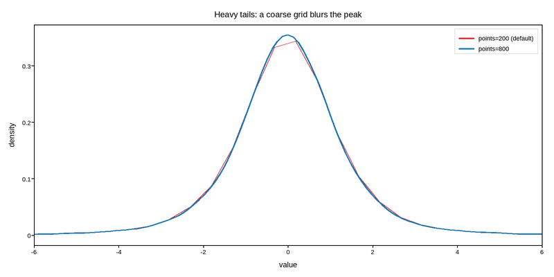
Binning is only as fine as the grid. When heavy-tailed outliers stretch the range, the default 200-point grid can be too coarse to resolve the peak, so it comes out slightly blocky. Raising points= refines the grid where you need it – the one knob worth reaching for on awkward data.

heavy = rng.standard_t(3, 50_000)          # extreme outliers stretch the range

fig2, ax = plotpress.subplots(figsize=(8, 4))
ax.kdeplot(heavy, points=200, color="#d62728", linewidth=1.0,
           label="points=200 (default)")
ax.kdeplot(heavy, points=800, color="#1f77b4", linewidth=1.8,
           label="points=800")
ax.set_xlim(-6, 6)                         # the bulk; outliers reach much further
ax.set_title("Heavy tails: a coarse grid blurs the peak")
ax.set_xlabel("value")
ax.set_ylabel("density")
ax.legend()
fig2.tight_layout()

Live figure — pick a tool, then zoom, pan, point-pick or annotate. Nothing is active until a tool is selected.

View this figure’s Vega export ↗ — the raw JSON spec, rendered live by a real Vega engine.

View this figure’s Vega-Lite export ↗ — the raw JSON spec(s), rendered live by a real Vega-Lite engine.

Both integrate to 1 and recover the same shape; the finer grid just resolves the peak more smoothly. For well-behaved data the default is already accurate to a fraction of a percent, so this is a knob for the awkward cases, not one you normally touch.